Calculating the Probabilities of a 100-Sided "Weighted" Dice

Question

I have always been interested in learning how I can make a custom Probability Distribution that corresponds to some particular situation (e.g. constraints).

For example - suppose I have a single dice that has 100 sides and the following conditions:

• Condition 1: This dice has the highest probability of landing on 50
• Condition 2: Sides closer to 50 have higher probabilities compared to sides farther away from 50 (i.e. monotonically strictly decreasing, e.g. Probability of landing on side 50 > 49 > 48 ... AND Probability of landing on side 50> 51 > 52 >...)
• Condition 3: Sides at equal distance to 50 have the same probabilities (e.g. Probability of landing on side 49 = Probability of landing on side 51, Probability of landing on side 48 = Probability of landing on side 52, etc.)

My Question: I want to make a separate dice that corresponds to each one of these situations below:

• Situation 1: I want to create a dice that satisfies Condition 1, Condition 2 and Condition 3. How can I define a Probability Distribution Function for this situation?
• Situation 2: I want to create a dice that satisfies Condition 1, Condition 2 and Condition 3 AND the probability of landing on side 50 is given by $p_{50} = 0.5$. How can I define a Probability Distribution Function for this situation?
• Situation 3: I want to create a dice that satisfies Condition 1, Condition 2 and Condition 3 AND the probability of landing on side 50 is given by $p_{50} = 0.5$ AND the probability of landing on side 49 = side 51 = 0.3. How can I define a Probability Distribution Function for this situation?

I am not sure how to solve these kinds of questions analytically. Ideally, I would be interested in defining an exact theoretical probability distribution corresponding to each situation (e.g. a multinomial distribution with certain properties).

What I tried so far: For the time being, I tried to solve this question by simulation (e.g. Situation 1). Using the R programming language, I simulated numbers from a Normal Distribution (centered around 50), truncated the results (i.e. only allowed numbers between 0 and 100), and calculated the probabilities of landing between any given ranges:

# define mean, standard deviation of a normal distribution with a large number of simulations
    mean <- 50
    sd <- 15
    n <- 100000
simulate from this normal distribution
set.seed(123)  
numbers &lt;- rnorm(n, mean, sd)


truncate the distribution (i.e. only keep numbers between 0 and 100)
numbers &lt;- ifelse(numbers &lt; 0, 0, ifelse(numbers &gt; 100, 100, numbers))


Define the intervals
min_interval <- seq(0, 99, by = 1)
max_interval <- seq(1, 100, by = 1)
count <- vector("numeric", length(min_interval))
percentage <- vector("numeric", length(min_interval))
Calculate the count and percentage of numbers in each interval
for (i in seq_along(min_interval)) {
    count[i] <- sum(numbers >= min_interval[i] & numbers < max_interval[i])
    percentage[i] <- count[i] / length(numbers) * 100
}
store results
df <- data.frame(min_interval = min_interval,
                 max_interval = max_interval,
                 count = count,
                 percentage = percentage)
#sort results
df <- df[order(-df$percentage), ]

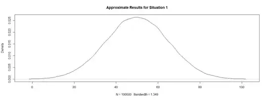
As we can see, the results of this simulation approximately correspond to Situation 1 (Condition 2 and Condition 3 are not fully met):

# plot results
plot(density(numbers))

We can see that numbers around 50 have higher probabilities (i.e. percentage/100) compared to numbers further away from 50 (even though Condition 2 and Condition 3 are not fully met):

# view results
head(df)
   min_interval max_interval count percentage
51           50           51  2714      2.714
49           48           49  2632      2.632
50           49           50  2628      2.628
53           52           53  2626      2.626
48           47           48  2615      2.615
54           53           54  2611      2.611
tail(df)
    min_interval max_interval count percentage
95            94           95    22      0.022
3              2            3    19      0.019
100           99          100    16      0.016
4              3            4    14      0.014
98            97           98    12      0.012
99            98           99    10      0.010

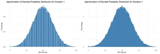
I also included an optional visualization:

library(ggplot2)
ggplot(df, aes(x=min_interval, y=percentage/100)) +
    geom_bar(stat="identity", fill="steelblue") +
    labs(x="Min Interval", y="Probability", title="Approximation of Discrete Probability Distribution for Situation 1") +
    theme_minimal()
ggplot(df, aes(x=min_interval, y=percentage)) +
    geom_bar(stat="identity", fill="steelblue", color="steelblue", width=1) +
    labs(x="Min Interval", y="Percentage", title="Approximation of Discrete Probability Distribution for Situation 1") +
    theme_minimal()

But is there a way to mathematically (i.e. analytically) calculate these probabilities for Situation 1, Situation 2 and Situation 3? Can a system of equations be created corresponding to Situation 1, Situation 2 and Situation 3 alongside a set of constraints - such that these probabilities can be calculated analytically? Perhaps this can be done with a Multinomial Distribution? Maybe an Exponential Decay Function that can be used such that it passes through all points?

Thanks!

• Notes:
• My own previous attempt at (incorrectly) approaching a similar question How to Define a Bell Curve
• Is this current question even possible? Will it require complex non-linear optimization algorithms?

Answer 1

The probabilities have to add up to $1$. Subtract any fixed probabilities e.g. $p_{50}=0.5$

The put $p_{1}=k, p_{2}=2k$ etc...

Then $2(k+2k+3k+....49k)=0.5$

$k=\frac{1}{4900}$ and make the 51, 52 etc... probabilities symmetrical with the 49,48 etc...

(the sum of numbers 1 to $n$ is $\frac{1}{2}n(n+1)$)

You can adjust this method depending on what central values are being fixed.

Answer 2

Situation 3 does not obey the laws of probability since $$p(50)+p(49)+p(51)=0.5+0.3+0.3=1.1$$

When creating a probability distribution, ensure normalization: the sum of probabilities in the sample space must be 1.

Situation 2 is asymmetrical and modelling analytically becomes more difficult: $$1<2<...<49: 49 \text{Outcomes}$$ $$5)<52<...<100: 50 \text{Outcomes}$$

With 101 outcomes, the modelling is easier:

Binomial Distribution with number of trials $=n=101$, and probability of success$=p=\frac{1}{2}$ gives a symmetric distribution with: $$p(1)<p(2)<...<p(50)<p(51), p(51)>p(52)>...>p(101)$$

Geometric Parameter Generalizing $p(51)=p, p(49)=p(52)=kp, p(48)=p(53)=k^2p$ gives: $$p(51-n)=p(51+n)=k^np$$

Summing all the probabilitites to 1 gives: $$p+k(2p)+k^2(2p)+...k^{50}(2p)=1$$

In your case $p(50)=p=0.5\Rightarrow2p=1$ $$0.5+k+k^2+...k^{50}=1$$ $$k+k^2+...k^{50}=0.5$$

This is now a geometric series with first term $k$, common ratio $k$, and 50 terms. Use the formula for the sum of a geometric series to find the value of $k$ and you are done.