Solving master equation for binding kinetics $\frac{dp_m(t)}{dt}=a\,(N-m+1)(M-m+1)p_{m-1}(t)+b\,(m+1)p_{m+1}(t)-[b\,m+a(N-m)(M-m)]p_m(t)$

Question

Background: This problem appears when you try solving the stochastic binding kinetics. There are a total of $M$ and $N$ molecules of the types $R$ and $L$. These molecules can be either in a bound ($RL$) or an unbound state. Each pair of unbound $R$ and $L$ molecules can bind with the rate $a$, and each bound molecule $RL$ can unbind with the rate $b$. Starting with $m_0$ initially bound pairs, I would like to find $p_m(t)$, the probability of having $m$ molecules in the bound state $RL$ at time $t$.

Problem: The following set of coupled differential equations (also known as Master equations) describe the dynamics of the probabilities $p_m(t)$ as functions of time $$ \frac{dp_m(t)}{dt}=a\,(N-m+1)(M-m+1)p_{m-1}(t)+b\,(m+1)p_{m+1}(t)-[b\,m+a(N-m)(M-m)]p_m(t), $$ where $M$ and $N$ are integers with $0<M\leq N$ and $a>0$ and $b>0$ are real numbers, for integer $m$s between $0\leq m\leq M$, with the initial conditions $p_m(0) = \delta_{m,m_0}$, $0\leq m_0\leq M$. Assume $p_{-1}(t)=p_{M+1}(t)=0$.

I would like to solve these equations.

What I tried so far: We can write the set of ODEs as a Matrix equation of the form $$ \frac{d}{dt}\left(\begin{array}{c} p_0\\ \vdots\\ p_M \end{array}\right)=\underbrace{\left(\begin{array}{cccc} -aNM&b &0&0&\dots\\ aNM&-b-a(N-1)(M-1) &2b&0&\dots\\ &\vdots \end{array}\right)}_{\mathbf{A}}\left(\begin{array}{c} p_0\\ \vdots\\ p_M \end{array}\right) $$ with the formal solution $\mathbf{p}(t)=e^{\mathbf{A}t}\mathbf{p}(0)$. But in order to exponential the matrix $t\mathbf{A}$, I need to diagonalize $\mathbf A$, but I don't know how to do that. It is a tridiagonal matrix, each column adds up to one, and it has a simple form. I'm sure someone on SE knows how to diagonalize this.

Alternatively, I tried solving the problem using a generating function defined as $$ f(z,t) = \sum_{m=0}^M p_m(t) z^m. $$ You can differentiate $f$ with respect to $t$ and find the following PDE satisfied by $f$: $$ \partial_t f = a(z-1)\left[MNf-\left((M+N-1)z+\frac{b}{a}\right)\partial_zf+z^2\partial^2_zf\right], $$ with the initial condition $f(z,0)=z^{m_0}$. But I do not know how to solve this equation either. It is a second-order linear PDE with a solution that is a polynomial in $z$, so it should be solvable.

Steady State Results: Binding kinetics has an equilibrium solution that is given by Boltzmann distribution with the partition function $$\mathcal{Z} = \sum_{m=0}^M \left(\frac ba\right)^m {M \choose m}{N \choose m}={}_2F_1(-M,-N,1,b/a).$$ This gives $$p_m(\infty) = \frac{\left(\frac ba\right)^m {M \choose m}{N \choose m}}{{}_2F_1(-M,-N,1,b/a)}.$$

What I need: Ideally looking for a closed-form solution for either $p_m(t)$ or $f(z,t)$. If there is no closed-form solution, at least an explicit expression for $p_m(t)$ that could involve special functions or maybe even a sum or series, but something that I can explicitly calculate. I'm not looking for a numerical solution.

Answer 1

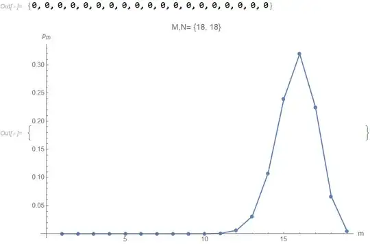
Alright. The steady state of the model can be relatively easily found.All what you need to do is to set the left hand side of your last equation to zero . then the resulting ODE is easy to solve because the term $(z-1)$ can be cancelled. The final result is as follows:

\begin{equation} p_m(\infty) = \left. \frac{1}{m!} \frac{d^m}{d w^m} \frac{w^M \, _1F_1\left(-M;-M+N+1;-\frac{b}{a w}\right)}{\, _1F_1\left(-M;-M+N+1;-\frac{b}{a}\right)} \right|_{w=0} \end{equation}

for $m=0,\cdots,M$. Here $N > M \ge 1$.

{NN, M} = RandomInteger[{10, 20}, 2]; If[NN < M, tmp = NN; NN = M; 
 M = tmp]; {a, b} = Rationalize[RandomReal[{0, 1}, 2], 1/1000]; w =.;
vecinf = Simplify[
    Table[D[w^M Hypergeometric1F1[-M, 1 - M + NN, -(b/(a w))]/
         Hypergeometric1F1[-M, 1 - M + NN, -(b/a )], {w, m}]/m!, {m, 
      0, M}]] /. w :> 0;
KK = Table[
   Which[n == m - 1, a (NN - m + 1) (M - m + 1), n == m + 1, 
    b (m + 1), n == m, -(b m + a (NN - m) (M - m)), True, 0], {m, 0, 
    M}, {n, 0, M}];
vec = Eigenvectors[KK][[-1]];
vec = vec/Total[vec];
vecinf - vec
{ListPlot[vecinf, PlotMarkers -> Automatic, Joined :> True, 
  AxesLabel -> {"m", Subscript[p, m]}, ImageSize -> 500, 
  PlotLabel -> "M,N= " <> ToString[{M, NN}]]}

---

Now, in order to solve the full problem we need to separate variables in your PDE and then find the solution to the spatial part . Here I do not know if it is possible to reduce the resulting equation to hypergeometric functions. All what I can say now is that the ODE we come across is of the same form as the second ODE listed here. It is very likely that the ODE in question will be reduced to the Heun equation but I wouldn't know how to do it now.

Answer 2

Hint.

Calling the generic ode after Laplace transformation

$$ (s+c_m)p_m + a_m p_{m-1}+b_m p_{m+1}=\phi_m $$

The ODE system can be displayed as

$$ \left(\matrix{ s+c_0&b_0&0&0&0&\cdots & 0 &0\\ a_1&s+c_1&b_1&c_3&0&\cdots & 0&0\\ 0&a_2&s+c_2&b_2&0&\cdots & 0&0\\ \vdots&\vdots&\vdots&\vdots&\vdots& &\vdots&\vdots\\ 0&0&0&0&0&\cdots&a_M&s+ c_M}\right)\left(\matrix{p_1\\ p_2\\ p_3\\ \vdots\\ p_M}\right) = \left(\matrix{\phi_1\\ \phi_2\\ \phi_3\\ \vdots\\ \phi_M}\right) $$

or

$$ M(s).p = \phi $$

where $\phi$ are the initial conditions.

The determinant of $M$ as tridiagonal, follows the continuant sequence. For this case

$$ \Delta_k = (s+c_k)\Delta_{k-1}-a_{k}b_{k-1} \Delta_{k-2} $$

with $\Delta_0=1, \Delta_{-1}=0$.

The characteristic polynomial can be easily computed (numerically) and also their roots giving thus the eigenvalues.

Regarding $\lim_{t\to\infty}p_m(t)$ this limit can be obtained directly by doing after knowing that $p_m(t)$ is stable.

$$ p_m(\infty) = \lim_{s\to 0}s p_m(s) $$

$M(s)$ can be symbolically inverted with the MATHEMATICA script (tridinv)

tridinv[a_?VectorQ, b_?VectorQ, c_?VectorQ] /; 
Length[b] - 1 == Length[a] == Length[c] := Module[{n = Length[b], p = a c, f, t}, t = FoldList[Dot, IdentityMatrix[2], 
 Transpose[{{Table[0, {n}], Table[1, {n}]}, {-Append[p, 0], b}}, {2, 3, 1}]][[All, 2, 2]];
 f = Reverse[FoldList[Dot, IdentityMatrix[2], 
  Transpose[{{Table[0, {n}], Table[1, {n}]}, {-Append[Reverse[p], 0], Reverse[b]}}, {2, 3, 1}]][[All, 2, 2]]];
  Table[(-1)^(i + j) t[[Min[i, j]]] f[[Max[i, j] + 1]] Product[Switch[Sign[i - j], -1, c[[l]], 0, 1, 1, a[[l]]], {l, Min[i, j], Max[i, j] - 1}], {i, n}, {j, n}]/t[[n + 1]]
]

so for $M = N = 6$ we have

M = 6;
NN = 6;
aa[m_] := -(a (M - m + 1) (NN - m + 1))
bb[m_] := -(b (m + 1))
cc[m_] := -(bb[m - 1] + aa[m - 1])
av = Table[bb[k], {k, 0, M - 1}]
bv = Table[s + cc[k], {k, 0, M}]
cv = Table[aa[k], {k, 1, M}]
iM = tridinv[av, bv, cv]

Thus, having the $\det(M(s))=0$ roots, we can build the $p_m(t)$ solutions.