2

I've had some idea I could do something like this:

$${\bf v_o}=\min_{\bf v} \{\|{\bf M(v+r)}\|_2^2 + \epsilon\|{\bf v}\|_2^2\}$$

for a random vector $\bf r$ and then $\bf v$ should point in the direction where $\bf M$ has largest eigenvalue because it is in the negative of that direction the norm will be squeezed the most. Then we can iterate this by setting $\bf r = r+v_o$ and resolving until $\bf v_0$ does not change and we should have a vector in the null space.


But the iteration kind of bugs me. It is inelegant. I would like to try and express and solve it all simultaneously in one big grande equation system. Any ideas?

mathreadler
  • 26,534

2 Answers2

3

Problem statement

Let's take a slightly different perspective on this problem and say that we start with the matrix $M\in\mathbb{C}^{m\times n}_{\rho}$, and a data vector $b\in\mathbb{C}^{m}$. This data vector isn't in the null space $\color{red}{\mathcal{N}\left(\mathbf{M}^{*}\right)}$. Finally, we possess the Moore-Penrose pseudoinverse, $\mathbf{M}^{+}$. That is, we have the least squares solution and that unlocks both left and right null spaces.

Building null space vectors

The solution provides access to vectors in both null spaces, $\color{red}{\mathcal{N}\left(\mathbf{M}^{*}\right)}$ (when $\rho < m$), and $\color{red}{\mathcal{N}\left(\mathbf{M}\right)}$ $(\rho < n)$.

The least squares problem $$ x_{LS} = \left\{ x\in\mathbb{C}^{n} \colon \lVert \mathbf{M} x - b \rVert_{2}^{2} \text{ is minimized} \right\} $$ has the general solution $$ x_{LS} = \color{blue}{\mathbf{M}^{+} b} + \color{red}{\left( \mathbf{I}_{n} + \mathbf{M}^{+}\mathbf{M} \right)y}, \qquad y \in \mathbb{C}^{n} $$ Subspace membership is color coded for $\color{blue}{range}$ and $\color{red}{null}$ spaces.

Right null space

The operator which projects an $n-$vector onto the null space $\color{red}{\mathcal{N}\left(\mathbf{M}^{*}\right)}$ is $$ \mathbf{P}_{\color{red}{\mathcal{N}\left( \mathbf{M}\right)}} = \color{red}{\left( \mathbf{I}_{n} + \mathbf{M}^{+}\mathbf{M} \right)} $$ Input a vector $y$ and output the projection of $y$ onto the right null space.

Left null space

The crucial insight here is to resolve the data vector in to range and null space components: $$ b = \color{blue}{b_{\mathcal{R}}} + \color{red}{b_{\mathcal{N}}} $$

The matrix pseudoinverse provides the projection of the data vector on the range space: $$ \color{blue}{b_{\mathcal{R}}} = \color{blue}{\mathbf{M}^{+}b} $$ A null space vector is then $$ \color{red}{b_{\mathcal{N}}} = b - \color{blue}{b_{\mathcal{R}}} = b - \color{blue}{\mathbf{M}^{+}b} $$

dantopa
  • 10,768
  • Calculating a pseudoinverse is quite demanding. The purpose of the algorithm would be to get a quick estimate for the eigenspace without having to calculate anything complicated like diagonalization or pseudoinverse. – mathreadler Sep 09 '17 at 19:22
1

After some experimentation it seems that $\bf M v_0$ estimates the largest eigenvector. My intuition tells me that the relation between $\bf r$ and this eigenvector should affect the quality of this estimate, but I can't really figure out the relationship. Maybe scalar products are a good start.


The experiment setup: $${\bf M}\in \mathbb R^{3\times 3}, \hspace{0.5cm}{\bf M}_{ij} = \mathcal N (\mu=0,\sigma=1) + 10\cdot {\bf vv}^T, \hspace{0.5cm}{\bf v} \in \mathbb R^{3\times 1}, {\bf v}_i = \mathcal N(\mu,\sigma=1)$$ After this ${\bf v}$ is normed to have $L_2$ norm 1.

Now doing: $${\bf v_0} = ({\bf M}^T{\bf M} + 10^3{\bf I})^{-1}(-2{\bf M}^T{\bf r} )$$

And then calculating the absolute value of the normed scalar product:

$$\frac 1 {\|{\bf Mv_0}\|} \cdot |<{\bf Mv_0}, {\bf v}>|$$ and stuffing into a histogram for 1024 different randomized $\bf r$:

enter image description here

In addition we have 2 straight-forward continuations


  1. Iterate the procedure for the found $\bf v_0$ to try and refine the estimate from last iteration.
  2. Solve for once for several $\bf v_0$ in parallel and then fuse the estimates.

The 2 is most straight forward to implement as we can expand column vectors $\bf v,r$ to matrices $\bf V,R$ where each column is a candidate eigendirection. Therefore we try it, also we choose to weight the candidate $\bf MV_0$ together using remappings of scalar products with $\bf R$ : $\text{diag}({\bf R}^T{\bf MV_0})^{\circ p}$ with $\circ p$ denoting Schur/Hadamard (elementwise) power function - and of course we must divide by the total sum. We leave out some practical details as for example make the internal scalar products positive so they don't give destructive interference in the weighted averaging. Let us call the averaged solution ${\bf V_{0s}}$.


Then what remains to find a complete eigensystem is to update the above system to forbid the previously found eigenvectors. Our approach here is to successively update the left hand side $\bf L$ and right hand side $\bf r$ by adding $${\bf L} \stackrel{+}{=} \epsilon {\bf V_{0s}}{\bf V_{0s}}^T\\{\bf r} \stackrel{+}{=} {{\bf M}^T \bf V_{0s}}$$ This will of course only be theoretically acceptable if we expect an orthogonal system of eigenvectors, but it's a start!

A typical "lucky" scalar product matrix we could get with 8 fused candidate directions for each eigenvector ( perfect would be $100 \cdot {\bf I}_3$ ): $$100\cdot {\bf S_0}^T{\bf S} \approx \left[\begin{array}{ccc} 100&-13&-1\\-4&100&1\\0&0&100\end{array}\right]$$

( $\bf S$ is the "true" matrix in ${\bf M} = {\bf SDS}^{-1}$ given by computer-language builtin "eig" command and $\bf S_0$ is the estimate given by our method. )

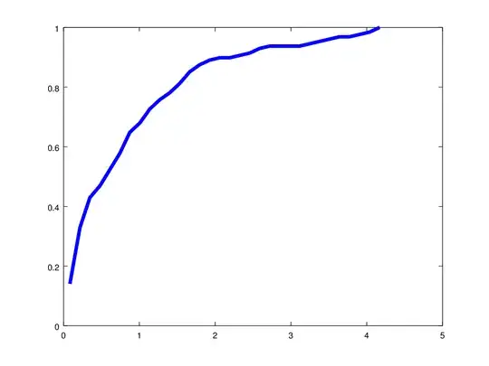
An accumulated error histogram (cumulative distribution function) using the error $\|{\bf S_0}^T{\bf S - I}_3\|_1$ (for our example above it is $\frac{13+1+4+1}{100} = 0.19$):

enter image description here

mathreadler
  • 26,534