What is minimum speed needed to jump over sphere object that has radius $R$ and at distance $d$?

Question

(I am not expert in English. I will write as well as I can.)

To understand this question easier, lets see this picture.

From this picture, what is minimum initial speed that this grasshopper need to jump over this log?

The grasshopper movement path can touch the log but can't cross through inside of the log.

$d$ and $R$ can be any positive real number which $d>R$. $g$ is a gravitational acceleration (approximately $9.80665 \, \mathrm{m/s^2}$).

This is a mathematical-physics question but mainly in maths.

I can do physics part but have problem in maths part.

Physics Part : Let red ball is grasshopper and at origin point and $y$ is height.

The relation between $x$ and $y$ for projectile motion is $$y(x) = x \tan\theta - \frac{gx^2}{2u^2 \cos^2\theta}, \quad 0 < \theta < \frac{\pi}{2}.$$

Upper curve of sphere can be described in function: $$y_s(x) = R + \sqrt{R^2-(x-d)^2}, \qquad \text{for} \quad d-R \leq x \leq d+R.$$

Condition of the sphere is $$y(x) \geq y_s(x), \qquad \text{for} \quad d-R \leq x \leq d+R$$ or

$$x \tan\theta - \frac{gx^2}{2u^2 \cos^2\theta} \geq R + \sqrt{R^2-(x-d)^2}, \qquad \text{for} \quad {d-R \leq x \leq d+R}.$$

At this point, I don't how to find $u_{\min}(d,R)$ from this.

(If you give values of $d$ and $h$ (for example, $d = 2 \, \mathrm{m}$ and $R = 1 \, \mathrm{m}$), it is possible to find $\theta$ that minimizes $u$.)

I know only $y(x)$ (parabola curve) for $u_{\min}(d,R)$ looks like that.

Case: $d = cR$ ($c$ is a constant. There is a ratio that make $y(x)$ have maximum point at the top of the sphere.)

Case: $d > cR$

Case: $d < cR$

Please help me.

Answer 1

This turns out to be an interesting question, but one which I believe is impossible to solve in closed form. However, you should be able to follow the steps I give and get a graphical/numerical solution.

As we know, the grasshopper will follow the trajectory $$y = (\tan\theta)x - \frac12 g\big(\frac x{u\cos\theta}\big)^2.$$ Lagrange multipliers tells us that it will intersect the circle $(x-d)^2+(y-R)^2=R^2$ tangentially at a point $(x,y)$ when $$\left(\tan\theta - \frac{gx}{(u\cos\theta)^2}, -1\right) = \lambda(x-d,y-R)$$ for some nonzero $\lambda$. Eliminating $\lambda$ gives us the equation $$g(x,y,u,\theta) = x\Big(\frac1{y-R}-\frac g{(u\cos\theta)^2}\Big) - \frac d{y-R} + \tan\theta = 0.$$ Consider the function $$F(x,y,u,\theta) = \big((x-d)^2+(y-R)^2-R^2,g(x,y,u,\theta)\big)$$ mapping an appropriate region in $\Bbb R^4$ to $\Bbb R^2$. We are interested in the zero set $F(x,y,u,\theta) = (0,0)$.

The implicit function theorem tells us that if the $2\times 2$ minor of the Jacobian of $F$ given by $\frac{\partial F}{\partial (x,y)}$ is nonzero, then on that zero set we can locally solve for $(x,y)$ as functions of $(u,\theta)$ on an open set. Since we are looking for a minimum possible $u$, we cannot allow $u$ to get any smaller, and hence there is no such local solution on an open set. We must therefore have $\frac{\partial F}{\partial (x,y)} = 0$. Working this out and substituting the equation $(x-d)^2+(y-R)^2=R^2$ where appropriate we should get $$R^2(u\cos\theta)^2 = g(y-R)^3 \tag{$\star$}.$$ We now have $y=y(u,\theta)$. Substituting ($\star$) in $g(x,y,u,\theta)=0$ will give (a messy) formula for $x$ as function of $(u,\theta)$. Using the equation $(x-d)^2+(y-R)^2=R^2$ once again, we will at last get an equation $h(u,\theta) = 0$.

Once again, we appeal to the implicit function theorem. If $\dfrac{\partial h}{\partial \theta}\ne 0$, we will, as before, get $\theta$ locally as a function of $u$ on an open interval of $u$ values. Since this, too, cannot happen when we've found the minimum $u$, we must have $$\frac{\partial h}{\partial \theta} = 0.$$ Substituting our values of $x(u,\theta)$ and $y(u,\theta)$ in this should, at least, give an equation that can be solved to give our minimum $u$.

Good luck!

Answer 2

Given a point $(c,s)$ on the unit circle $c^2+s^2 = 1$,
we obtain a point $(x = d+cr, y = r+sr)$ on the circle,
then we find the parabola $y = -ax^2+bx$ that is tangent to that point by solving the system of equations $y = -ax^2+bx, c = 2asx-bs$.

Doing so, we get $a = \frac{sy+cx}{sx^2}, b =\frac{2sy+cx}{sx}$.

And from there, the energy of the grasshopper during his jump is proportional to $\frac{b^2+1}a$, so the goal is to find $(c,s)$ that minimizes this.

If we parametrize the unit circle with $c = \frac{t^2-1}{t^2+1}, s = \frac {2t}{t^2+1}$ and do all the computations,

we obtain $\frac {b^2+1}a = \frac{(r+d)^2t^6 + 8r(r+d)t^5 + (31r^2+18dr+3d^2)t^4 + 48r^2t^3 + (31r^2-18dr+3d^2)t^2 + 8r(r-d)t + (r-d)^2}{2t(t+1)(t^2+1)((r+d)t+(r-d))}$.

I have checked that this is a degree $6$ rational fraction, so this is its reduced form, and so the minimum is obtained when the derivative of this with respect to $t$ vanishes, so after some more computation, when this polynomial

$P_{r,d}(t) = (r+d)^3t^{10}+4r(r+d)^2t^9-3(r+d)^2(3r+d)t^8-8r(r+d)(7r-d)t^7 \\ -(74r^3-50r^2d-46rd^2+14d^3)t^6+144r^2dt^5+(74r^3+50r^2d-46rd^2-14d^3)t^4 \\ +8r(r-d)(7r-d)t^3+3(r-d)^2(3r-d)t^2-4r(r-d)^2t-(r-d)^3$

vanishes. Now, how complicated is this thing ?

The discriminant of this has degree $3 \times 19$ in $r,d$, and it almost factors nicely over the integers :

$\Delta = d^{10} r^4 (d^2+r^2)^2 (d-r)^8 (d+r)^{11} (d-2r)(d+2r)\\ (64d^6+144d^4r^2+81d^2r^4+27r^6) (d^6-2d^4r^2-2d^2r^4-r^6)^2$

After looking at the monodromy when $r/d$ makes a small circle around all of those points, you get permutations of the roots, then if you follow paths to a common point, you can gather them up and obtain generators for the Galois group of the extension, which turns out to be $S_4 \times S_6$ : the degree $10$ polynomial wasn't irreducible (!)

Forming the irreducible factors is easy once you have the orbits of the roots under the Galois group and so now after drawing lots of pictures and doing many more computations, we have :

$P_{r,d}(t) = Q_{r,d}(t) R_{r,d}(t) = \\ ((r+d)t^4 + 4rt^3-6dt^2-4rt-(r-d))\\ ((r+d)^2t^6-3(r+d)(3r-d)t^4-16r^2t^3-3(r-d)(3r+d)t^2+(r-d)^2) $

Now, to identify which root corresponds to the minimum we want, things get a bit weird. In general the energy blows up four times on the real axis : when the trajectory is a line, so at $t=-1$ (then the trajectory is the $x$-axis), at the other tangent $t = t_{d/r} = (d-r)/(d+r)$, and when the grasshopper jumps vertically to infinity before falling down in a vertical tangent line, at $t= 0$ and $t = \infty$. Obviously we are interested only in the interval $(t_{d/r} ; \infty)$

If $r > 2d$, the only root of the derivative in that interval is a root of the quartic $Q_{r,d}$. This root gives us the solution we want. Also, note that as $r/d \to \infty$, this root converges to $\sqrt{3+\sqrt 8}$.

If $r = 2d$, the sextic $R_{r,d}$ has a double root that pops up at $t=1$.

If $r < 2d$, the roots of the sextic give a local maximum and a second local minimum. However, their corresponding parabolas fail to jump over the circle as they intersect it transversally at some other places.

Finally, at $r/d = k \approx 1.9$, the solution from the quartic becomes bitangent to the circle.

If $r < kt$, then the two local minima both fail to jump over the ball, so the solution we want is no longer a local minimum of the energy, but is the parabola that's bitangent to the ball.

This happens when the expression $(x-d)^2 + ((-ax^2+bx)-r)^2 - r^2$ is a square.

$(x-d)^2 + ((-ax^2+bx)-r)^2 - r^2 \\ = a^2x^4 - 2abx^3 + (2ar+b^2+1)x^2 - (2br+2d)x + d^2 \\ = (-ax^2 + bx - r - \frac 1 {2a})^2 + (\frac ba-2d)x + (d^2-(r+ \frac 1 {2a})^2))$

Hence $\frac ba-2d = 0$ and $d^2-(r+\frac 1 {2a})^2 = 0$. We need to pick the positive solution $a = \frac 1{2(d-r)}$, then $b = 2da = \frac d {d-r}$

Now I want to find the exact value of $k$, so when $r/d$ is such that those two solutions coincide.

Continuing from the bitangent solution, the tangent points now happen at the two roots of $-ax^2 + bx - r - \frac 1 {2a}$. After replacing $a,b$ with their values, this becomes equivalent to $x^2 - 2dx +2d(d-r)$, so $(x-d)^2 = (2r-d)d$.

Thus, $c^2r^2 = (2r-d)d$, and so $(t^2-1)^2r^2 = (t^2+1)^2(2r-d)d$, and we ge the equation $(r-d)^2 t^4 +2(d^2-2dr-r^2)t^2 + (r-d)^2 = 0$

Taking its resolvant with the other quartic gives a degree $12$ polynomial in $r,d$, which factors as $(d-r)^2d^2(2d^4-6d^3r+6d^2r^2-8dr^3+9r^4)(2d^4-6d^3r+6d^2r^2-4dr^3+r^4)$

This has some interesting real roots for $r/d$, in particular it gives $k \approx 1.90340819201887$, one of the roots of the second quartic, so $2k^4-6k^3+6k^2-4k+1 = 0$

Answer 3

For $R<d\le 2R$ and symmetrical contact (two contact points, on either side of circle)

$\hspace{1cm}$

Consider the case where the parabola (projectile trajectory) touches the circle (cross section of sphere) at two points, $A, B$. Let these points subtend an angle $\theta$ to the vertical at the centre of the circle.

Take the contact point between the circle and ground as the origin.

Let $V(0,h)$ be the point of intersection of the tangents (to both trajectory and circle) at $A,B$. By simple trigonometry, it can be easily worked out that $h=R\left(1+\frac 1{\cos\theta}\right)$ Hence the three points are

$$A\big(-R\sin\theta, R(1+\cos\theta)\big); \qquad V\big(0,R\left(1+\tfrac 1{\cos\theta}\right)\big); \qquad B\big(R\sin\theta, R(1+\cos\theta)\big)$$ Hence the parametric form of the parabola can be stated as a quadratic Bezier curve as follows:

$$\begin{align} (x,y) &=\bigg(t^2(-R\sin\theta+2t(1-t)\cdot 0+(1-t)^2(R\sin\theta)\; ,\\ &\qquad t^2 R(1+\cos\theta)+2t(1-t)R(1+\tfrac 1{\cos\theta})+(1-t)^2R(1+\cos\theta) \bigg)\\ &=\bigg(\ (1-2t)R\sin\theta\; ,\;(1-2t+2t^2)R(1+\cos\theta)+2t(1-t)R(1+\tfrac 1{\cos\theta})\ \bigg)\end{align}$$ Eliminating $t$ gives the Cartesian form of the trajectory $$\boxed{y=\frac {R^2(1+\cos\theta)^2-x^2}{2R\cos\theta}}\\ \text{which is equivalent to }\\ \boxed{\frac {x^2}{R^2(1+\cos\theta)^2}+\frac y{\left(\frac {R^2(1+\cos\theta)^2}{2R\cos\theta}\right)}=1}$$ As the launch point is given as $(-d,0)$, this gives $$d=R(1+\cos\theta)\Longrightarrow \cos\theta=\tfrac dR-1$$ Hence the equation of the trajectory becomes $$\boxed{y=\frac {d^2-x^2}{2(d-R)}}\\ \scriptsize(R<d\le 2R)\\ \text{which is equivalent to}\\ \boxed{\frac {x^2}{d^2}+\frac y{\left(\frac{d^2}{2(d-R)}\right)}=1}\\ \frac {dy}{dx}=-\frac x{d-R}=\frac d{d-R}\text{ at } x=-d$$ Let $v, \alpha$ be the launch velocity and launch angle respectively.
Hence $$\boxed{\tan\alpha =\frac d{d-R}}$$
Equating coefficients of $x^2$ with the standard trajectory equation $y=x\tan\alpha-\frac {gx^2}{2v^2}(1+\tan^2\alpha)$ gives $$\begin{align} \frac 1{2(d-R)} &=\frac g{2v^2}(1+\tan^2\alpha)\\ &=\frac g{2v^2}\big(1+\left(\tfrac d{d-R}\right)^2\big)\\ \color{red}{v^2}&\color{red}{=gd\left(\frac d{d-R}+\frac {d-R}d\right)} \qquad \scriptsize (R<d\le 2R) \end{align}$$

Another method:

Parabola: $$\frac {x^2}{d^2}+\frac yh=1\tag{1}$$ Circle: $$x^2+(y-R)^2=R^2\tag{2}$$ $d^2\times (1)-(2)$: $$\begin{align} (y-R)^2-\frac {d^2}hy&=R^2-d^2\\ y^2-(2R+\tfrac{d^2}h)y+R^2=R^2-d^2\\ y^2-\left(\frac {2Rh+d^2}h\right)y+d^2&=0\\ \text{For tangency, } \left(\frac {2Rh+d^2}h\right)^2&=4d^2\\ \frac {2Rh+d^2}h&=\pm 2d\\ h&=\frac {d^2}{2(d-R)}\end{align}$$ Hence equation for parabola is $$\boxed{y=\frac {d^2-x^2}{2(d-R)}}$$ and the rest follows per above.

---

For $d\ge 2R$ and symmetrical contact (one contact point, at top of circle)

For this case where $d\ge 2R$, the launch point is sufficient far enough to just touch the top of the circle without hitting any other part. Hence this is the same as a projectile with its vertex of its trajectory at the top of the circle.

Using standard formulas for maximum height and range of a projectile, we have

$$\begin{align} 2R&=\frac {v^2}{2g}\sin^2\alpha\qquad(1)\\ d&=\frac {v^2}{2g}\sin 2\alpha\qquad(2)\\ (1)/(2):\hspace{1cm}\frac{2R}d&=\frac {\tan\alpha}2\\\end{align}$$ $$\boxed{\tan\alpha=\frac {4R}d}\\$$ $$\begin{align}\text{From }(2):\hspace{1cm}\\ d&=\frac {v^2}{2g}\cdot \frac {2\tan\alpha}{1+\tan^2\alpha}\\ \color{red}{v^2}&\color{red}{=gd\left(\frac {d}{4R}+\frac{4R}d\right)} \qquad \scriptsize (d\ge 2R) \end{align}$$

The equation of the parabola is $$\boxed{\frac{x^2}{d^2}+\frac y{2R}=1}\\ \text{which is equivalent to}\\ \boxed{y=2R\left(1-\frac {x^2}{d^2}\right)}$$

---

See Desmos implementation here.

Answer 4

I do not believe your approach is the simplest.

The height of the jump is:

$$ 2R = \frac{\dot y_0^2}{2g} $$

So: $$ \dot y_0 = \sqrt{Rg} $$

Now take each component separately. First, what is the minimal vertical speed needed to jump a height of 2R? As in he will get to 2R and start falling. So, his velocity will be zero at a height of 2R. Use the equation:

$$ \dot y_{2R} = 0 = \dot y_0 - gt$$ $$ t = \frac{\dot y_0}{g}$$

This is the time to get a height of 2R in gravity. Well, the grasshopper has to travel $d = \dot x t$ in this time so:

$$ t = \frac{d}{\dot x} $$

Solving for $\dot y_0$ and $\dot x$ and substituting t where appropriate yields:

$$\dot y_0 = t \cdot g = \frac{d \cdot g}{\dot x} $$ $$ \dot x =\frac{d}{t} = \frac{d \cdot g}{\dot y_0} $$

Substitute $\dot y_0$ from above: $$ \dot x = \frac{d \cdot g}{\sqrt{Rg}} $$

The rest is up to you. You have your two components in terms of $R$, $g$, and $d$.

Answer 5

Minimum initial speed $\; \to \; $
$\; \to \;$ minimal kinetic energy at start ($E=1/2mv^2=1/2m({v_h}^2+{v_v}^2=E_h+E_v$) $\; \to \;$
$\; \to \;$ minimal vertical kinetic energy at start $E_v$ (the horizontal translation speed and energy are unaffected) $\; \to \;$
$\; \to \;$ minimal potential energy at top $\; \to \;$ minimum $h$.

Given the vertex and a point (the starting one), the parabola is fully determined: therefore the minimum $h$ corresponds to the parabola tangent to the given circle.

To simplify the calculations let's invert the representation as in the second part of the sketch above, and let's consider the parabola $y=ax^2$.

A circle will be internally bi-tangent to the parabola if its center lies on the axis and on the normal to the parabola.
The tangent to the parabola at a point $(x_0,a{x_0}^2)$ has a slope of $2a{x_0}$, so the slope of the normal is $-1/(2a{x_0})$.
So if we impose that the center be at $(0,h)$, on the normal and at distance $R$ from the parabola, we get $$ \left\{ \matrix{ {{h - a\,x_{\,0} ^{\,2} } \over {x_{\,0} }} = {1 \over {2\,a\,x_{\,0} }} \hfill \cr \left( {h - a\,x_{\,0} ^{\,2} } \right)^{\,2} + x_{\,0} ^{\,2} = R^{\,2} \hfill \cr} \right.\quad \Rightarrow \quad \left\{ \matrix{ h = a\,R^{\,2} + {1 \over {4\,a}} \hfill \cr x_{\,0} ^{\,2} = R^{\,2} - {1 \over {4\,a^{\,2} }} \hfill \cr} \right. $$ that says that the bi-tangent circle of radius $R$ has the center at $h=1/(4a)+aR^2$.
See also this related post.

Imposing then that parabola passes through the starting point $(-d, R+h)$, and solving for $a$ $$ \eqalign{ & \left\{ \matrix{ h = {1 \over {4\,a}} + a\,R^{\,2} \hfill \cr R + h = a\,d^{\,2} \hfill \cr} \right.\quad \Rightarrow \quad \left\{ \matrix{ 4R^{\,2} \,a^{\,2} - 4\,ah + \,1 = 0 \hfill \cr R + h = a\,d^{\,2} \hfill \cr} \right.\quad \Rightarrow \cr & \Rightarrow \quad \left\{ \matrix{ 4R^{\,2} \,a^{\,2} - 4\,ah + \,1 = 0 \hfill \cr h = a\,d^{\,2} - R \hfill \cr} \right.\quad \Rightarrow \cr & \Rightarrow \quad \left( {d^{\,2} - R^{\,2} } \right)\,a^{\,2} - \,R\,a - \,1/4 = 0 \cr} $$ which means $$ \eqalign{ & a = {{R \pm \sqrt {R^{\,2} + \left( {d^{\,2} - R^{\,2} } \right)} } \over {2\left( {d^{\,2} - R^{\,2} } \right)}}\, = {{R \pm d} \over {2\left( {d^{\,2} - R^{\,2} } \right)}} = \cr & = {{R \pm d} \over {2\left( {d + R} \right)\left( {d - R} \right)}} = \left\{ \matrix{ {1 \over {2\left( {d - R} \right)}} \hfill \cr - {1 \over {2\left( {d + R} \right)}} \hfill \cr} \right. \cr} $$

We are interested to the positive solution, therefore the final result is $$ \bbox[lightyellow] { \left\{ \matrix{ a = {1 \over {2\left( {d - R} \right)}} \hfill \cr h = a\,d^{\,2} - R = {{\left( {d - R} \right)^{\,2} + R^{\,2} } \over {2\left( {d - R} \right)}} \hfill \cr x_{\,0} ^{\,2} = R^{\,2} - \left( {d - R} \right)^{\,2} \hfill \cr R \le d \le 2R \hfill \cr} \right. }$$

where :

• if $d \to R$, then clearly $h$ and $a$ go to infinity while $x_0$ becomes $R$;

• if $d \to 2R$, then the circle has radius $R=1/(2a)$ equal to the curvature at the vertex of the parabola, $h$ becomes $R$ and will remain so if $d$ increases over $2R$.

And of course, once you have the parabola's parameters defined (and flipped back to the original sketch), it's easy to assess the minimum initial speed and elevation angle.

I think that the simplest way is just to "flip" the $g$ and then consider that the vertical speed shall be taken to be positive.

So, indicating by $T$ the time to reach the top (bottom), by $u$ and $v$ the horizontal and vertical velocities, we shall have $$ \left\{ \matrix{ u\,T = d \hfill \cr g\,T = v \hfill \cr {{g\,T^2 } \over 2} = R + h = a\,d^{\,2} = {{d^{\,2} } \over {2\left( {d - R} \right)}} \hfill \cr} \right. $$ and finally, always for $\bbox[lightyellow] { R \le d \le 2R}$, all the needed parameters are easily obtained:

$$ \bbox[lightyellow] { \left\{ \matrix{ a = {1 \over {2\left( {d - R} \right)}} \hfill \cr R + h = {{d^{\,2} } \over {2\left( {d - R} \right)}} \hfill \cr T = {d \over {\sqrt {g\left( {d - R} \right)} }} \hfill \cr u\, = \sqrt {g\left( {d - R} \right)} \hfill \cr v = {{g\,d} \over {\sqrt {g\left( {d - R} \right)} }} \hfill \cr \tan \theta = {v \over u} = {{\,d} \over {\left( {d - R} \right)}} \hfill \cr u^{\,2} + v^{\,2} = g\left( {2d + {{\,R^{\,2} } \over {\left( {d - R} \right)}}} \right) \hfill \cr} \right. }$$

That gives the parametric equation in time as $$ \bbox[lightyellow] { \left\{ \matrix{ y(t) = R + h - {1 \over 2}g\left( {t - T} \right)^2 = d\sqrt {{g \over {d - R}}} \;t - {1 \over 2}g\,t^2 \hfill \cr x = u(t - T) = - d + \sqrt {g\left( {d - R} \right)} \;t \hfill \cr} \right. }$$ which in fact turns into $$ \bbox[lightyellow] { y(x) = R + h - {1 \over 2}g\left( {{x \over u}} \right)^2 = R + h - a\,x^2 = {{d^2 - x^2 } \over {2\left( {d - R} \right)}} }$$

Answer 6

We need to find a relation for $v_{min}$ in terms of $(d,R,g) $ using the geometry of the parabola and kinematics of a projectile /grasshopper that projects itself up.

Finding the parabola trajectory height $H$

The Subnormal SN has a constant length of projection $=2f$ projected from TN on axis. This can also be computed in another way: $$(x,y)= (2ft, ft^2) ,~ t=\tan \phi~,~ 2 f \sin \phi/\cos \phi = R \sin \phi~$$ $$ R= 2f \sec \phi, ~ R \cos \phi = 2f \tag1$$ Maximum height of grasshopper's jump $H$ $$ H= R+R \cos \phi +f \tan ^2 \phi $$ Plugging in from (1) and simplifying, $$ H= f (1+\sec \phi)^2 \tag 2$$ Eliminating $ \sec \phi$ from (1) and (2) $$H=\frac{(2f+R)^2}{4f} \tag 3 $$ Parabola equation $$ H=\frac{d^2}{4f} \tag 4 $$ Eliminating $f$ with algebraic simplification between (3) and (4) results in $$ H=\frac{d^2}{2(d-R)} \tag 5 $$ Parabola property: Since $ UV=VB=h,$ $$\tan A = \frac{2H}{d}, \sin A = \frac{2H}{\sqrt{4 H^2-d^2}},~\sin^2A= \frac{4H^2}{4H^2-d^2} \tag 6 $$ Plugging in from (5) into (6) and simplifying $$ \sin^2 A= \left (2-2\frac{R}{d}+\frac{R^2}{d^2}\right) \tag 7 $$ Uniform motion along vertical symmetry line

Upward uniform motion along parabola line of symmetry is considered. The velocity decelerates to zero in a height of $H$. Using standard kinematic relation $$(v \cdot\sin A)^2 -0^2=2 g H \tag 8 $$ and simplifying we finally have $$ v =d^2\sqrt{\frac{g}{(d-R)(2d^2-2dR+R^2)}}\tag 9 $$ To find $v_{min}$ we differentiate the above as a function of $d$ w.r.t. $d$ using the Quotient Rule to simplify: $$\frac{d^4}{2d^3-4 d^2 R+3 d R^2-R^3}= \frac{4d^3}{6 d^2 -8 d R +3 R^2 } $$ $$ u= \frac{d}{R},~ 2 u^3 -8 u^2 + 9 u -4 =0 \to u= \frac{d}{R}\approx 2.537 \tag {10}$$

In a numerical example for a log of radius $R=1$ meter,$ \text{d=2.537 meters, H = 2.0938 meters, given g=9.81 meter/sec^2 };$

We finally have

$$ v_{min} \approx 5.482~\text{meters/sec.} $$

Answer 7

We will approach this problem two fold.

$A-$Two contacts between the path and the circle. $\left(\frac dr \le 1.375\right)$

$B-$One contact between the path and the circle. $\left(1.375\lt \frac dr\right)$

For the first case, we will use a tangency technique and for the second case, a Lagrange multipliers formulation.

Case $A$:

Giving

$$ \cases{ y = a x + b x^2\\ (x-d)^2+(y-r)^2= r^2 } $$

eliminating $y$ we get

$$ p(x)=d^2-2 d x-2 a r x+a^2 x^2-2 b r x^2+x^2+2 a b x^3+b^2 x^4=0 $$

Now, having two tangent points $(x_1,x_2)$ then should be true for $\forall x$, that $p(x)=k(x-x_1)^2(x-x_2)^2$ or

$$ \left\{ \begin{array}{rcl} d^2-k x_1^2 x_2^2 & = &0\\ -2 a r-2 d+2 k x_1^2 x_2+2 k x_1 x_2^2 & = & 0 \\ a^2-2 b r-k x_1^2-4 k x_1 x_2-k x_2^2+1 & = & 0\\ 2 a b+2 k x_1+2 k x_2 & = & 0\\ b^2-k & = & 0\\ \end{array} \right. $$

Solving we get

$$ \cases{ k=\frac{1}{4 (d-r)^2}\\ x_1=d-\sqrt{d (2 r-d)}\\ x_2=d+\sqrt{d (2 r-d)}\\ a=\frac{d}{d-r}\\ b=-\frac{1}{2 (d-r)} } $$

We know also that

$$ \cases{ a = u\tan\theta\\ b = -\frac{g}{2u^2\cos^2\theta} } $$

so for $1\le \frac dr\le 1.375$ we can use this formulation to solve the problem.

Case $B$:

Here the problem is solved using the lagrangian

$$ \cases{ g_1(x,y,u,s,c) = y- u \frac sc x + \frac{g x^2}{u^2c^2} = 0\\ g_2(s,c) = s^2+c^2-1 = 0\\ g_3(x,y) = (x-d)^2+(y-r)^2-r^2 = 0\\ L(x,y,u,s,c,\lambda_i,\mu,\delta) = u + \lambda_1g_1(x.y,u,s,c)+\lambda_2 g_2(s,c) + \lambda_3 g_3(x,y)+\lambda_{4,5}\left(\nabla_{x,y}g_1 - \mu\nabla_{x,y}g_3\right)+\lambda_6\left(\frac sc-\frac{2\tan(r/d)}{1-\tan²(r/d)}-\delta^2\right) } $$

Here, the last constraint, reveals that the start angle understood as $\theta^*$, obeys $ = \arctan(s^*/c^*) > \arctan\left(\frac{2\tan(r/d)}{1-\tan²(r/d)}\right)$

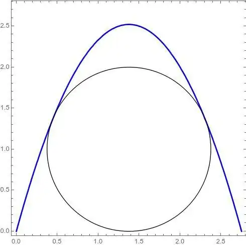
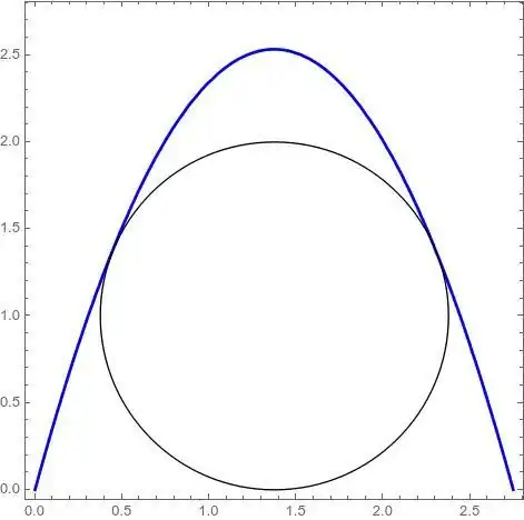
Follows a MATHEMATICA script illustrating the cases $A$ and $B$

(*****************************)
(**  for 1 <= d/r <= 1.375  **)
(*****************************)
Clear[k]
g1 = y - (a x + b x^2);
g2 = (x - d)^2 + (y - r)^2 - r^2;
g3 = First[Eliminate[{g1 == 0, g2 == 0}, y]] - k (x - x1)^2 (x - x2)^2;
coefs = CoefficientList[g3, x];
sols = Quiet@Solve[coefs == 0, {k, x0, x1, x2, a, b}];
parms = {d -> 1.375, r -> 1, g -> 10};
solb = Solve[g (a^2 + u^2) == -2 b u^4, u][[2]];
sols0 = {u, a, b} /. solb /. sols /. parms;
choosed = {};
For[k = 1, k <= Length[sols0], k++, 
  If[RealValuedNumberQ[N[sols0[[k, 1]]]], 
   AppendTo[choosed, sols0[[k]]]]];
choosed = Sort[choosed];
choosed // N
g10 = g1 /. Thread[{a, b} -> {choosed[[1, 2]], choosed[[1, 3]]}] /. parms;
Show[ContourPlot[g10 == 0, {x, 0, 2 d} /. parms, {y, 0, 2 d} /. parms], Graphics[Circle[{d, r}, r] /. parms], PlotRange -> {{0, 2 d}, {0, 2 d}} /. parms, ImageAspectRatio -> 1]

(*****************************)
(**    for 1.375 <= d/r     **)
(*****************************)
g1 = y - u  sin/cos x + 1/2 g x^2/u^2/cos^2;
g2 = (x - d)^2 + (y - r)^2 - r^2;
g3 = sin^2 + cos^2 - 1;
L = u + lambda1 g1 + lambda2 g2 + lambda3 g3 + {lambda4, lambda5}.(Grad[g1, {x, y}] - mu Grad[g2, {x, y}]) + lambda6 (sin/cos - N[2 Tan[r/d]/(1 - Tan[r/d]^2)] - s^2);
vars = {x, y, u, t, sin, cos, lambda1, lambda2, lambda3, lambda4, lambda5, lambda6, mu, s};
equs = Grad[L, vars];
parms = {g -> 10, d -> 1.375, r -> 1};
equs0 = equs /. parms;
sols = Quiet@Solve[equs0 == 0, vars];
nsols = Length[sols];
psols = {u, ArcTan[sin/cos], (2 u^3 cos sin)/g} /. parms /. sols /. {C[1] -> 0} // N;
choosed = {};
For[k = 1, k <= nsols, k++, 
 If[RealValuedNumberQ[psols[[k, 1]]] && psols[[k, 3]] > ((d + r) /. parms) && psols[[k, 1]] > 0, AppendTo[choosed, psols[[k]]]]]
choosed = Sort[Union[choosed]]
grfs = ContourPlot[((y - u Tan[t] x + 1/2 g x^2/u^2/Cos[t]^2) /. parms /. Thread[{u, t} -> {choosed[[1, 1]], choosed[[1, 2]]}]) == 0, {x, 0, 2 d} /. parms, {y, 0, 2 d} /. parms, ContourStyle -> {Blue, Thick}];
Show[grfs, Graphics[Circle[{d, r}, r] /. parms], PlotRange -> {{0, 2 d}, {0, 2 d}} /. parms, ImageAspectRatio -> 1]

Unresolved question: how to determine exactly the transition point between procedures? $(1.375...)$

Answer 8

In my understanding,'d' is irrelevant for finding the minimum speed required to jump over a sphere or pipe of radius R. To actually accomplish the jump however, 'd' will be relevant. But easiest way to solve this problem (just for finding launch speed) is to consider an angle 'theta' that determines the fist point of contact of the insect with the circular surface, and then use projectile motion concepts plus a little bit of calculus to find the minimum launch speed. I have solved this question in a video for a student, which I posted on youtube (sorry but its in English and Hindi mixed). A screenshot of that video solution screenshotsolution is attached.YOUTUBE video solution