Abstract
The problem statement has:
$y=mx+b$ that giving the minimal value for the function $w=\sum_{i=1}^n (mx_i+b-y_i)^2$.
I need to prove that $w$ maintains:
$$b=\frac{\sum_{i=1}^n x_i^2\sum_{i=1}^ny_i -\sum_{i=1}^nx_i\sum_{i=1}^nx_iy_i}{n(\sum_{i=1}^nx_i^2)-(\sum_{i=1}^nx_i)^2 }$$ and: $$\\m=\frac{n(\sum_{i=1}^nx_iy_i-\sum_{i=1}^nx_i \sum_{i=1}^ny_i}{n\sum_{i=1}^nx_i^2-(\sum_{i=1}^nx_i)^2}$$
In the problem statement, $m$ is the slope and $b$ is the intercept.
Hence, in the question:
$$\text{Intercept }=\frac{\sum_{i=1}^n x_i^2\sum_{i=1}^ny_i -\sum_{i=1}^nx_i\sum_{i=1}^nx_iy_i}{n(\sum_{i=1}^nx_i^2)-(\sum_{i=1}^nx_i)^2 }$$ and: $$\\\text{Slope }=\frac{n(\sum_{i=1}^nx_iy_i-\sum_{i=1}^nx_i \sum_{i=1}^ny_i}{n\sum_{i=1}^nx_i^2-(\sum_{i=1}^nx_i)^2}$$
In the step-by step derivation below using slightly different variables $y=a+bx$, where below $a$ is the intercept and $b$ is the slope, the same result is derived that:
$$
\text{Intercept }=\frac
{
-
\left(
\sum_{i=1}^{i\le n } x_i*x_i
\right)
*\left(
\left(
\sum_{i=1}^{i\le n } y_i
\right)
\right)
+
\left(
\sum_{i=1}^{i\le n } x_i
\right)
*
\left(
\left( \sum_{i=1}^{i\le n } y_i*x_i \right)
\right)
}
{
\left(
\sum_{i=1}^{i\le n } x_i*x_i
\right)
*
\left(
-n \right)
-
\left(
\sum_{i=1}^{i\le n } x_i
\right)
*
\left(
- 1*
\left(
\sum_{i=1}^{i\le n } x_i
\right)
\right)
}
\tag{15}
$$
$$\text{Slope }=\frac
{-\left( \sum_{i=1}^{i\le n } x_i \right)
\left(
\left( \sum_{i=1}^{i\le n } y_i \right)
\right) +
\left(
n*\left(\left( \sum_{i=1}^{i\le n } y_i*x_i \right)
\right)
\right)}
{
\left( \sum_{i=1}^{i\le n } x_i \right)\left(-1*\left(\sum_{i=1}^{i\le n } x_i \right)\right) + \left(
n*\left(\sum_{i=1}^{i\le n } x_i*x_i\right)\right)
}
\tag{14}$$
And this result is correct as it also duplicates the result for the slope from the reference (expanding the relevant sums):
$$
\text{Slope }=\frac{n*\left(\sum x_i*y_i\right)-\left(\sum x_i \sum y_i \right)}
{n \sum{\left(x_i\right)^2} - \left( \sum{x_i} \right)^2}
\tag{16}$$
Succinct Derivation of the Standard Linear Regression Approach
This derivation leans heavily on the succinct answers here. But it adds a little bit more detail so that it is a little bit more obvious how to go from step to step, so that it is obvious whether the answer is correct or not. I am considering how to extend the result for linear regression, so I want to make sure to understand each and every step fully.
I do admire the answer from "SA-255525". But I prefer to work the problem out step-by-step to be able to troubleshoot any mistakes. The steps are too large there for me to be able to assert the correctness of that answer.
I also reference at the bottom an answer that is the same final result! I have a spreadsheet or I can use a program, so it is easy for me to calculate floating sums and divisions to further test the reults.
First, the the error $w=\sum_{\text{error squared}}$ be defined as follows:
$$w=\sum_{i=1}^{i<i_{right}}\left(y_i-\left(a+b*x_i\right)\right)^2\tag{1}$$
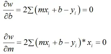
Now there are two variables to solve for, namely $a$ and $b$. And there are two equations, since the derivative of $w$ with respect to $a$ and $b$ needs to be zero at an inflection point, like a maximum or minimum. The reference proves that this zero point is the minimum error and not the maximum. Hence:
$$w=\sum_{i=1}^{i<i_{right}}\left(y_i-\left(a+b*x_i\right)\right)^2$$
$$\frac{d w}{d a} = \frac {d \sum_{i=1}^{i<i_{right}}\left(y_i-\left(a+b*x_i\right)\right)^2}{d a}=0\tag{2}$$
$$= -2 \sum_{i=1}^{i<i_{right}}\left(y_i-\left(a+b*x_i\right)\right)$$
$$= 0 \text{ at the maximum point for a}$$
$$\underset{\text{implies}}{\longrightarrow}\sum_{i=1}^{i<i_{right}}\left(y_i-\left(a+b*x_i\right)\right)=0
$$
$$\underset{\text{implies}}{\longrightarrow}
\text{ (with }n=i_{right}-1) \text{ that }\left( \sum_{i=1}^{i\le n } y_i \right) - b*\left(\sum_{i=1}^{i\le n } x_i \right)-n*a=0\tag{3}
$$
Dividing Equation 3 by $n$, defining $\bar{y}=\frac{\sum_{i=1}^{i\le n}{y_i}}{n}$, $\bar{x}=\frac{\sum{x_i}_{i=1}^{i \le n}}{n}$, and setting terms that are not $\bar{y}$ to the right side of the equation immediately results in the widely quoted (definitely correct) result:
$$
\bar{y}=a+b*\bar{x}
$$
Also, the derivative $\frac{ d w}{d b}=0$ at the minimum and hence:
$$\frac{d w}{d b} = \frac {d \sum_{i=1}^{i\le n}\left(y_i-\left(a+b*x_i\right)\right)^2}{d b}=0\tag{4}$$
Then,
$$\frac{d w}{d b}= -2 \sum_{i=1}^{i\le n}\left(y_i-\left(a+b*x_i\right)\right)*x_i=0$$
And similarly it follows that:
$$\text{ (with }n=i_{right}-1) \text{ that }\left( \sum_{i=1}^{i\le n } y_i*x_i \right) - b*\left(\sum_{i=1}^{i\le n } x_i*x_i\right) - a \left( \sum_{i=1}^{i\le n } x_i \right)=0\tag{5}
$$
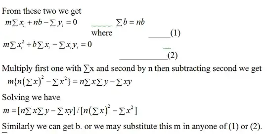
To solve for $b$, by elimination $a$ from Equations 3 and 5, Equation 3 is multiplied by $\left( \sum_{i=1}^{i\le n } x_i \right)$ resulting in Equation 6; and Equation 5 is multiplied by $n$ resulting in Equation 7. And then the modified second Equation 7 is subtracted from the modified first Equation 6 so to solve for $b$ in Equation 8 as follows:
$$\left( \sum_{i=1}^{i\le n } x_i \right)\left(\left( \sum_{i=1}^{i\le n } y_i \right) - b*\left(\sum_{i=1}^{i\le n } x_i \right)\right) -\left(\left(\sum_{i=1}^{i\le n } x_i \right)*n*a\right)=0\tag{6}
$$
$$n*\left(\left( \sum_{i=1}^{i\le n } y_i*x_i \right) - b*\left(\sum_{i=1}^{i\le n } x_i*x_i\right)\right) - \left( \left( \sum_{i=1}^{i\le n } x_i \right ) *n*a \right)=0\tag{7}
$$
$$\left( \sum_{i=1}^{i\le n } x_i \right)\left(\left( \sum_{i=1}^{i\le n } y_i \right) - b*\left(\sum_{i=1}^{i\le n } x_i \right)\right) - \left(
n*\left(\left( \sum_{i=1}^{i\le n } y_i*x_i \right) - b*\left(\sum_{i=1}^{i\le n } x_i*x_i\right)\right)
\right)$$
$$
=0\tag{8}
$$
By manipulation of Equation 8, $b$ can be easily solved for. Equation 3 and Equation 5 can also be used by appropriate multiplications and subtractions to solve for $a$.
To solve for $a$, by elimination $b$ from Equations 3 and 5, Equation 3 is multiplied by $\left( \sum_{i=1}^{i\le n } x_i*x_i \right)$, resulting in Equation 9. And Equation 5 is multiplied by $\left( \sum_{i=1}^{i\le n } x_i \right)$, resulting in Equation 10. Then the modified second Equation 10 is subtracted from the modified first Equation 9 so solve for $a$ in Equation 11 as follows:
$$\left( \sum_{i=1}^{i\le n } x_i*x_i \right)*\left(\left( \sum_{i=1}^{i\le n } y_i \right) - b*\left(\sum_{i=1}^{i\le n } x_i \right)-n*a \right)=0\tag{9}
$$
$$\left( \sum_{i=1}^{i\le n } x_i \right)*
\left(
\left( \sum_{i=1}^{i\le n } y_i*x_i \right) - b*\left(\sum_{i=1}^{i\le n } x_i*x_i\right) - a \left( \sum_{i=1}^{i\le n } x_i \right)
\right)
=0\tag{10}
$$
$$\left( \sum_{i=1}^{i\le n } x_i*x_i \right)*\left(\left( \sum_{i=1}^{i\le n } y_i \right) -n*a \right)
-
\left( \sum_{i=1}^{i\le n } x_i \right)*
\left(
\left( \sum_{i=1}^{i\le n } y_i*x_i \right) - a \left( \sum_{i=1}^{i\le n } x_i \right)
\right)$$
$$=0\tag{11}
$$
For solving $b$, Equation 8 can be rearranged by putting the terms that include $b$ on the left of the equals sign and those remaining are multiplied by $-1$ on the right resulting in Equation 12 as follows:
$$
\left( \sum_{i=1}^{i\le n } x_i \right)\left(- b*\left(\sum_{i=1}^{i\le n } x_i \right)\right) - \left(
- n*b*\left(\sum_{i=1}^{i\le n } x_i*x_i\right)\right)
$$
$$=-\left( \sum_{i=1}^{i\le n } x_i \right)
\left(
\left( \sum_{i=1}^{i\le n } y_i \right)
\right) +
\left(
n*\left(\left( \sum_{i=1}^{i\le n } y_i*x_i \right)
\right)
\right)\tag{12}$$
For solving $a$, Equation 11 can be rearranged by putting the terms that include $a$ on the left of the equals sign and those remaining are multiplied by $-1$ on the right resulting in Equation 13 as follows:
$$
\left(
\sum_{i=1}^{i\le n } x_i*x_i
\right)
*
\left(
-n*a \right)
-
\left(
\sum_{i=1}^{i\le n } x_i
\right)
*
\left(
- a
\left(
\sum_{i=1}^{i\le n } x_i
\right)
\right)
$$
$$
=
-
\left(
\sum_{i=1}^{i\le n } x_i*x_i
\right)
*\left(
\left(
\sum_{i=1}^{i\le n } y_i
\right)
\right)
+
\left(
\sum_{i=1}^{i\le n } x_i
\right)
*
\left(
\left( \sum_{i=1}^{i\le n } y_i*x_i \right)
\right)
\tag{13}
$$
Now $b$ can be solved from Equation 12, by collecting all the terms on the left that include $b$ and dividing both sides of the equation by them, resulting in Equation 14:
$$b=\frac
{-\left( \sum_{i=1}^{i\le n } x_i \right)
\left(
\left( \sum_{i=1}^{i\le n } y_i \right)
\right) +
\left(
n*\left(\left( \sum_{i=1}^{i\le n } y_i*x_i \right)
\right)
\right)}
{
\left( \sum_{i=1}^{i\le n } x_i \right)\left(-1*\left(\sum_{i=1}^{i\le n } x_i \right)\right) + \left(
n*\left(\sum_{i=1}^{i\le n } x_i*x_i\right)\right)
}
\tag{14}$$
Similarly $a$ can be solved from Equation 13, by collecting all the terms on the left that include $a$ and dividing both sides of the equation by them, resulting in Equation 15:
$$
a=\frac
{
-
\left(
\sum_{i=1}^{i\le n } x_i*x_i
\right)
*\left(
\left(
\sum_{i=1}^{i\le n } y_i
\right)
\right)
+
\left(
\sum_{i=1}^{i\le n } x_i
\right)
*
\left(
\left( \sum_{i=1}^{i\le n } y_i*x_i \right)
\right)
}
{
\left(
\sum_{i=1}^{i\le n } x_i*x_i
\right)
*
\left(
-n \right)
-
\left(
\sum_{i=1}^{i\le n } x_i
\right)
*
\left(
- 1*
\left(
\sum_{i=1}^{i\le n } x_i
\right)
\right)
}
\tag{15}
$$
To check this result, start with the Reference: Derivation of the formula for Ordinary Least Squares Linear Regression. As to why it is important to reproduce the steps, it is to later have the capacity to expand them to non-linear regions also, perhaps here if not elsewhere.
The reference has the model $y_i=m*x_i+b$ versus here $y_i=a+b*x_i$ is the model applied. It is straightforward enough to adapt the Reference to what is used in the derivation here. And the result is the same. Adapted from the reference:
$$
b=\frac{n*\left(\sum x_i*y_i\right)-\left(\sum x_i \sum y_i \right)}
{n \sum{\left(x_i\right)^2} - \left( \sum{x_i} \right)^2}
\tag{16}$$
$$
a=\frac{\sum{y_i} - a* \sum{x_i}}
{n}
\tag{17}$$