Surprisingly good approximation of $\frac{x-1}{\ln x}$

Question

Today I was experimenting with numerical methods for a physics simulation and stumbled upon an approximation for this function that seems surprisingly accurate, given how simple it is. Basically, I found $$\frac{x-1}{\ln(x)} \approx \frac{2}{3} \sqrt{x} + \frac{1}{3} \frac{x+1}{2}.$$ An alternative way of stating this is $$\frac{a-b}{\ln(a)-\ln(b)} \approx \frac{2}{3} \sqrt{ab} + \frac{1}{3} \frac{a+b}{2}.$$ The expression on the right is a specific combination of the geometric and arithmetic mean of $a$ and $b$, which is how I discovered this by chance. I made a plot of the function and its approximation

with the relative error in green. My question is simply, why is this such a good approximation?

Answer 1

WLOG assume $a<b$. Using Simpson's 1/3 rule, we have: $$\frac{a-b}{\ln a-\ln b}=\int_{0}^{1}a^t b^{1-t}\,\mathrm dt\approx \frac{1}{6}\left(a+4\sqrt{ab}+b\right)=\frac{2}{3}\sqrt{ab}+\frac{1}{3}\frac{a+b}{2}$$ The error term is: $$|R|=\left|-\frac{1}{2880}\frac{d^4}{d\xi^4}a^\xi b^{1-\xi}\right|=\frac{1}{2880}a^\xi b^{1-\xi}\left(\ln a-\ln b\right)^4$$ for some $0\le \xi\le 1$. When $b>a$, applying AM-GM: $$\xi a+(1-\xi)b\ge a^\xi b^{1-\xi}$$ $$\implies |R|\le \frac{1}{2880}\left(\xi(a-b)+b\right)\left(\ln a-\ln b\right)^4\le \frac{1}{2880}b\left(\ln a-\ln b\right)^4$$ Consider the same for $a>b$ and combining, we get: $$|R|\le \frac{1}{2880}\left(\xi(a-b)+b\right)\left(\ln a-\ln b\right)^4\le \frac{1}{2880}\max(a,b)\left(\ln a-\ln b\right)^4$$ This might explain why.

Answer 2

This is an interesting approximation.

Trying to improve it up to $x=e^3$ and keeping the same form $$\frac{x-1}{\log(x)} \approx a \sqrt{x} + b(x+1)$$ consider the norm $$\Phi(a,b)=\int_0^{e^3} \Bigg(\frac{x-1}{\log(x)}-a \sqrt{x}- b(x+1) \Bigg)^2\, dx$$ which is fully explicit in terms of the exponential integral function and the logarithmic integral function.

Computing the partial derivatives with respect to $a$ and $b$ lead to a system of two linear equations and the result is fully explicit.

Converting to decimals and making them rational $$a\sim \frac{217}{309}\qquad \text{and} \qquad b \sim \frac{80}{523}$$

Comparing to your results $$\Delta_a= \frac{217}{309} -\frac 23=\frac{11}{309}\qquad \implies \text{relative error =}1.3\text{%}$$ $$\Delta_b= \frac{80}{523}-\frac 16=-\frac{43}{3138}\qquad \implies \text{relative error =}8.6\text{%}$$

The errors on the parameters are not large but their differences have a large impact. Using $12$ as an upper bound as in your plot, the norms are $5.25\times 10^{-3}$ and $3.65\times 10^{-4}$ and the absolute errors at the upper bound are $0.0493$ and $0.0056$.

Edit

Using, as @JohnBentin did in his answer, $$f_\lambda(x)=\lambda\sqrt x+\frac{1-\lambda} 2(x+1)\quad(0\leqslant\lambda\leqslant1;\,x>0)$$ we can use the same procedure as above for $0\leq x \leq e^3$ and obtain, converting the explicit value to decimals, $$\lambda_{\text{opt}}=0.686318 \sim \frac 2 3 + \frac 1{50}$$ whci explain why your approximation is so good.

For $x=12$, the absolute error is reduced to $0.0103$ and the infinite norm is $1.21\times 10^{-3}$.

Answer 3

We will show first that, of all approximants $$f_\lambda(x):=\lambda\surd x+(1-\lambda)\cdot\tfrac12(x+1)\quad(0\leqslant\lambda\leqslant1;\,x>0)$$ to $(x-1)/\ln x$, for $x$ near $1$, the best is when $\lambda=\frac23$. For convenience, write $t:=x-1$, where $t$ is small, and consider the relative error of the reciprocal functions: $$\varepsilon_\lambda(x):=\frac{f_\lambda(x)\ln x}{x-1}-1=\frac{f_\lambda(1+t)\ln(1+t)-t}t.$$ Using the usual binomial/Taylor expansions for $\surd(1+t)$ and $\ln(1+t)$, we get $$\begin{align}\varepsilon_\lambda(x) &=\frac{\left[1+\tfrac12t-\tfrac18\lambda t^2+O(t^3)\right]\left[t-\tfrac12t^2+\tfrac13t^3+O(t^4)\right]-t}t\\ &=-\tfrac14t^2+\tfrac13t^2-\tfrac18\lambda t^2+O(t^3)\\ &=\tfrac18(\tfrac23-\lambda)t^2+O(t^3).\end{align}$$ Clearly, this is minimized when $\lambda=\frac23$.

To look at the size of the error for $\lambda=\frac23$, we need to take the series to a higher order. It turns out that the approximation is actually better than $O(t^3)$, since the coefficient of $t^3$ in the expansion is $-\frac14+\frac16+\frac1{24}+\frac1{24}=0.$ If my calculation is correct, the error term is then $-\frac{121}{576}t^4+O(t^5)$.

Remark$\;$ This explains why the approximation is excellent for $x\approx1$, but not why it continues to be notably good even for sizeable values of $x$: for example, the error is still less than $1$% when $x=10$. Thinh Dinh's answer gives a more useful error bound for such larger values.

Answer 4

I figure some historical context may be of interest. The computation in the question is a particular instance of Borchardt's algorithm. This algorithm can be considered as a generalization of Archimedes' algorithm for the approximation of $\pi$ via inscribed and circumscribed regular polygons. I have pointed to the primary sources for this algorithm by Pfaff, Gauss, Schwab ^[1], and Borchardt in a previous answer on this site. The algorithm is defined by two linked sequences:

$$a_{i+1} = \frac{1}{2} \left(a_{i}+b_{i}\right)$$ $$b_{i+1} = \sqrt{a_{i+1}b_{i}}$$

If for $m \gt n$, one sets $a_{0}=m$ and $b_{0}=n$, then for $i \to \infty$, the $a_{i}$ and $b_{i}$ converge to a common limit

$$\omega =\frac{\sqrt{m^{2}-n^{2}}}{\cosh^{-1}\left(\frac{m}{n} \right)} $$

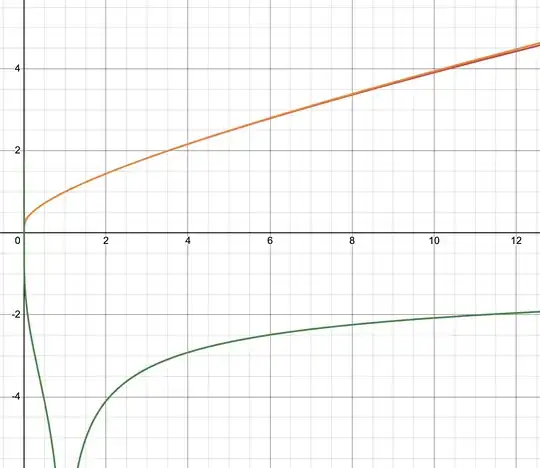
If, for $x > 1$, one sets $m=\frac{1}{2}(x+1)$ and $n=\sqrt{x}$, then $\omega = \frac{x-1}{\log(x)}$, which is precisely the function from the question.

For $m < n$ the common limit is instead

$$\omega =\frac{\sqrt{n^{2}-m^{2}}}{\cos^{-1}\left(\frac{m}{n} \right)} $$

illustrating the extension from the trigonometric space to the hyperbolic space provided by the algorithm. Borchardt's algorithm converges slowly, reducing the error relative to $\omega$ by only a factor of four per iteration. In both trigonometric and hyperbolic variants, the interpolation $\frac{1}{3}a_{n}+\frac{2}{3}b_{n}$ provides useful convergence acceleration: for any particular chosen error limit the variant using interpolation requires only half the number of iterations needed without the use of interpolation.

For the earlier algorithm of Archimedes and it sequences of inscribed and circumscribed polygons awareness of this interpolation goes back at least to Huygens' 1654 publication De circuli magnitudine inventa. In his theorem IX he states that (tr. Hazel Pearson, M.A. thesis, Boston University 1922) "the circumference of a circle is less than two-thirds the perimeter of the equilateral inscribed polygon plus one third the perimeter of a similar circumscribed polygon."

---

^[1] As Schwab's independent work is not as often credited as that of his better-known mathematical colleagues, I will give a brief outline here. Given a regular $n$-gon with perimeter $P$, and each side $S = P / n$, the radius of the inscribed circle is

$$ a = r_{inscribed} = P / (2 n \tan (\pi / n)) = S / (2 \tan (\pi / n)) $$

while the radius of the circumscribed circle is

$$ b = r_{circumscribed} = P / (2 n \sin (\pi / n)) = S / (2 \sin (\pi / n))$$

Jacques Schwab, "Élémens de géométrie". Nancy: C.-J. Hissette 1813, p. 104, presented the following result based on a geometric proof:

Let $a$ and $b$ be the radii of the inscribed and circumscribed circles of a regular $n$-gon with perimeter $P$. Then the corresponding quantities $a'$ and $b'$ of a regular $2n$-gon with the same perimeter $P$ are:

$$ a' = (a + b) / 2 $$ $$ b' = \sqrt{a' * b} $$