See update at end for extended simulations, and how these indicate that the average may diverge for all $p>0$. I see this is also the conclusion that Srini is leaning towards.
To fix a notation, let $X_{i,j}$ correspond to $\binom{i+j}{i}$ in the sense that $X_{i,0}=X_{0,j}=1$ and
$$
X_{i,j}=
\begin{cases}
X_{i-1,j}+X_{i,j-1} & \text{with probability $p$}\\
|X_{i-1,j}-X_{i,j-1}| & \text{with probability $1-p$}
\end{cases}
$$
for $i,j\ge1$, and where row $n$ of Pascal's triangle consists of $X_{i,j}$ for $i+j=n$.
First, we may note that the two alternatives are identical modulo 2: ie, which $X_{i,j}$ are odd or even is not random.
Next, if $p>1/2$, the expected value of $X_{i,j}$ is at least $p\cdot(X_{i-1,j}+X_{i,j-1})$, and so
$$
E\left[\sum_{i+j=n} X_{i,j}\right]
\ge 2p\cdot E\left[\sum_{i+j=n-1} X_{i,j}\right]
$$
which makes the expected average increase exponentially. I'm sure this could be extended to $p=1/2$ and maybe below by taking into account the variability of the values.
My next thought was to analyse $X_{i,j}$ for fixed $i$. For example, $X_{1,j}$ is a sequence that randomly increases or decreases by 1, and so in the long run there will be a distribution of values: ie it will converge to a probability distribution if $p<1/2$. This approach could be extended to $(X_{1,j},\ldots,X_{r,j})$, and we could ask for which $p$ this will converge towards an equilibrium distribution. However, before getting properly started on this analysis, I made some interesting discoveries.
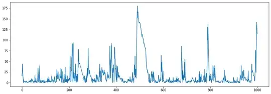
When making plots of $X_{i,j}$ for fixed $i$, I saw that when $p$ was low, ie well below $1/2$, the average was dominated by large spikes, while most of the $X_{i,j}$ would tend to remain small. Eg here is a segment $X_{14,5000..6000}$ from a simulation with $p=0.2$:
Spikes can arise by chance through a pattern of heads (when values are added), and then these spikes tend to carry on to subsequent values. This can be seen in a heatmap for $p=0.11$ where values have been transformed by $\log_2(X+1)$ for better illustration:
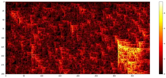
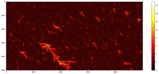
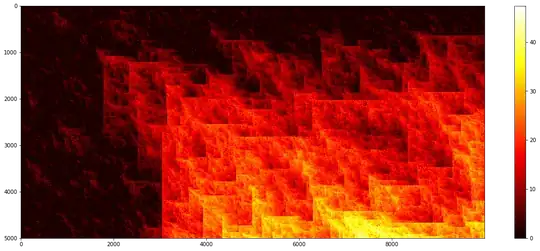
So, what drives the averages is how frequently these spikes arise, and how long they continue, which depends on $p$. Here is a case with $p=0.092$. The average value is just $9.3$, but this is primarily due to a small portion of values that are much larger.
 Note that the scale of the heatmap varies from map to map. Due to the logarithmic scale, a difference of $10$ on the scale corresponds to a factor of appr $1000$.
Since the spikes are highly sporadic, you will have to run the simulation for a while to see the long term behaviour, particularly for small $p$. Here is a case for $p=0.095$ for which the average values is $1358.4$, and it seems like the average is set to increase indefinitely as it keeps running:
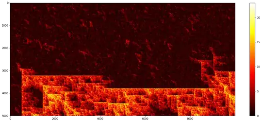
Here is a case of $p=0.10$ where the increase is even clearer:
I zoomed in on a $120\times60$ region from a $20000\times10000$ simulation with $p=0.09$ which shows one out of two major blow-up points in that simulation. Note that the colour scale here shows the actual values, ie not log-transformed as in the previous maps.

I looks as if when a certain pattern arises, a blow-up is almost inevitable, and once that happens it will spread out and thus eventually dominate the triangle. If that is true, the effect of $p$ is just to influence how long it takes for that pattern to occur, but no matter how rare it is, it will eventually take over, and so the average value will eventually diverge (with probability 1).
One way to think about this is that, if at some point there is a spike value, say of size $A$, with other values being mostly small, this starts what is basically a new random triangle but with values $A$ times as large. Then, you can get another random spike within this with an even grater value, and so on. However, it does seem like it takes a while for the initial spikes to appear, but then subsequent values tend to grow more quickly.
Update
I coded it in C to be able to do longer and bigger simulations, and the mean seems to start diverging even as $p$ gets below $0.09$. Here are a few results:
100000 x 100000 Pascal with p = 0.085000
Final mean = 21397033537218698805248.000000
Total mean = 851727491377168532897792.000000
250000 x 1000000 Pascal with p = 0.080000
Final mean = 29375911547.915989
Total mean = 79375851.833287
1000000 x 1000000 Pascal with p = 0.080000
Final mean = 62104889838672863782624815384565539227294683665492982388038245023744.000000
Total mean = 33037472267506384764204401071820950891726503895517883310943854657536.000000
Beware that, since spikes are now quite infrequent, the simulations have to run for a long time. The total mean is across all $N\times M$ values while the final mean is just the final column.
I am increasingly inclined to believe that the average will eventually start diverging whenever $p>0$, that it is just a matter of how long it takes for spikes to appear.
The simulations were written in Python and run in Jupyter with plots made using the matplotlib.pyplot package. Here is the core code:
import random
from math import log
from matplotlib import pyplot as plt
class Pascal(list):
    "Generates random array [0..d][0..n]"
    def init(self, p, n=1000, d=1):
        self.p = p
        self.n = n+1
        self.append([1]*self.n)
        self.increase(d)
def incdim(self):
    XX = self[-1]
    X, x = [], 1
    for i in range(self.n):
        y = XX[i]
        x = x+y if random.random()<self.p else abs(x-y)
        X.append(x)
    self.append(X)

def increase(self, d):
    for _ in range(d+1-len(self)):
        self.incdim()


Plot single diagonal
P = Pascal(0.2, 10000, 100)
X = P[14]
trans = lambda x: x  # Untransformed values
#trans = lambda x: log(1+x)/log(2)  # Log-transformed values
plt.figure(figsize=(15,5))
plt.plot([trans(_) for _ in X[5000:6000]])  # Segment of X selected
Heatmap
R, N = 2, 5000  # Size RN x N
off = 0  # Trim the first off columns/rows (keep ratio)
Q = Pascal(0.095, RN, N)
D = [[log(1+x)/log(2) for x in X[off:-1-(R-1)*off]] for X in Q[off:]]
plt.figure(figsize=(20,8))
plt.imshow(D, cmap='hot', interpolation='nearest')  # Heatmap
plt.colorbar()  # Adds a legend to show intensity
If run stand-alone, ie not in Jupyter, you probably have to add plt.show() after each plot to display them.


