I will solve the problem using an iterative method.
In 2D the constraint set for $\alpha = 0.4$ is given by:
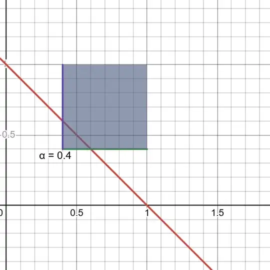
It is a convex set as @AlexShtoff pointed out.
One easy way to solve the problem is the Projected Gradient Descent.
One need two components to solve this:
- The Gradient
- The Projection onto the Constraints Set
The Gradient
The function is given by:
$$ f \left( \boldsymbol{x} \right) = -\boldsymbol{1}^{T} \boldsymbol{x} + \boldsymbol{1}^{T} \boldsymbol{y} - \boldsymbol{1}^{T} \left( \boldsymbol{x} \odot \ln \left( \boldsymbol{x} \right) - \boldsymbol{x} \odot \ln \left( \boldsymbol{y} \right) \right) $$
Hence the gradient is given by:
$$ \nabla f \left( \boldsymbol{x} \right) = \ln \left( \boldsymbol{x} \right) - \ln \left( \boldsymbol{y} \right) $$
Projection onto Unit Simples with Minimum Boundary Constraint
Similar to Orthogonal Projection onto the Unit Simplex.
With the difference being the function to find its root is given by:
$$ h \left( \mu \right) = \sum_{i = 1}^{n} { \left( {y}_{i} - \mu \right) }_{+\alpha} - 1 $$
Where ${ \left( x \right) }_{+\alpha} = \max \left\{ x, \alpha \right\}$.
Since $h \left( \cdot \right)$ is a piece wise linear function it should be evaluated at its joints which are given by ${y}_{i} - \mu = \alpha$.
Hence the evaluation points are ${y}_{i} - \alpha$.
Then the rest is as the case of $\alpha = 0$ as linked.
This is a 2D solution:
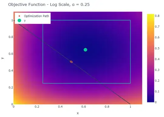
The code is available on my StackExchange Mathematics GitHub Repository (Look at the Mathematics\Q4834628 folder).

