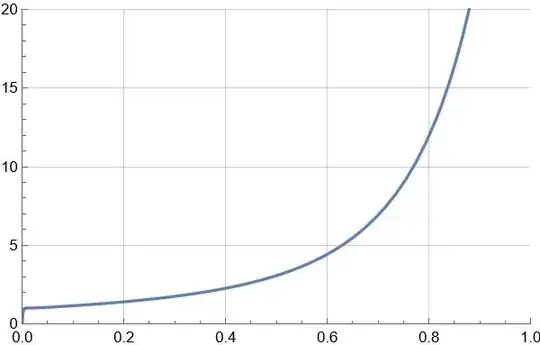
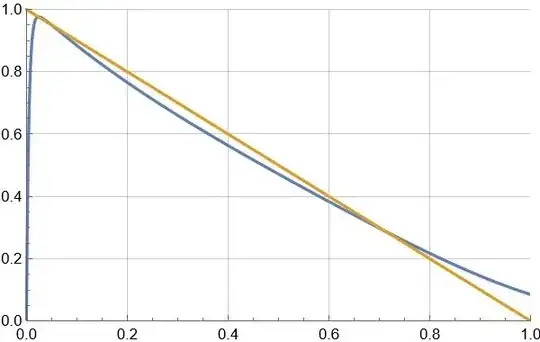
12

Say, we have $n$ positive i.i.d. random variables, $X_1, X_2, \dots, X_n$ which are distributed according to some probability distribution, $f$. So, only distributions on either $[0, 1]$ or $[0, +\infty]$.

The expected value of the ratio between the square of the sum and the sum of squares is then a function of $n$ and the distribution $f$,

$$ G(n; f) = \mathbb{E}\left[\frac{\left(\sum_{i=1}^{n} X_i\right)^2}{\sum_{i=1}^{n} X_i^2 } \right] $$

In general, I am interested in the behavior of this function, especially in the large-$n$ limit, or as $n \to \infty$. Specifically, for which distributions is $G(n; f)$ asymptotically constant?

It's easy to see that $G(n)$ is invariant to scaling such as $X_i \to a X_i$. So, there is no loss of generality when limiting ourselves to either distributions on $[0, 1]$ or $[0, +\infty]$. However, I suspect that it is not possible to get constant $G$ at large-$n$ for distributions on bounded intervals, anyway.


Here's how far I've gotten myself:

Firstly, we know that $1 \le G(n) \le n$ by the Cauchy-Schwarz inequality. $G(n) = n$ is only true for the Dirac delta distribution ($X_i = 1$).

It seems for some common distributions I tried out numerically, $G(n; f) \propto n$ in the large-$n$ limit. For example, with the uniform distribution, as $n \to \infty$

$$ G(n; U(0, 1)) \sim \frac{3}{4} n$$

I used some very non-rigorous manipulation ("physicist math"), assuming that the expected value of the ratio is the ratio of expected values in the large-$n$ limit, to derive

$$ G(n; f) \sim \frac{\mu^2}{\mu^2 + \sigma^2} n$$

where $f$ is a distribution with mean $\mu$ and variance $\sigma^2$. Numerically, this seems to agree with the uniform and log-normal distributions. My guess is that it applies to any distribution with finite mean and variance.


Numerically, I also found that for power-law distributions with heavy tails (such as Pareto distribution with $\alpha < 1$), $G(n)$ does appear to converge to a constant. But I can't seem to show this mathematically or find an expression for $G(n)$ in terms of $\alpha$.

Edit: An interesting, perhaps useful result from Albrecher & Teugels (2007), is that if $f$ is a Pareto-type distribution with $0 < \alpha < 1$, then

$$\lim_{n\to\infty} \mathbb{E}\left[\frac{\sum_{i=1}^{n} X_i^2 }{\left(\sum_{i=1}^{n} X_i\right)^2}\right] = {1 - \alpha} $$

Sangchul Lee
  • 181,930
XYZT
  • 1,065
  • Comments have been moved to chat; please do not continue the discussion here. Before posting a comment below this one, please review the purposes of comments. Comments that do not request clarification or suggest improvements usually belong as an answer, on [meta], or in [chat]. Comments continuing discussion may be removed. – Xander Henderson Aug 30 '23 at 15:12

5 Answers5

4

In this answer, we

  1. prove that $\frac{G(n, f)}{n} \to \frac{\mathbf{E}[X]^2}{\mathbf{E}[X^2]} $ whenever $\mathbf{E}[X] < \infty$, and

  2. show that $G(n, f)$ converges to some constant for some distribution $f$.

The statement and proof of each of the above claims will be demonstrated below, but let me make some informal remarks first.

The asymptotic behavior of $G(n, f)$ is determined by the survival function $R(t) = \mathbf{P}(X > t)$, which measures how much the distribution of $X$ is heavy-tailed. Indeed, $G(n, f)$ grows more slowly when $f$ is more heavy-tailed (or $R(t)$ decays more slowly). A heuristic computation shows:

  1. If $R(t)$ decays fast enough so that $\mathbf{E}[X^2] < \infty$, then $G(n,f) \asymp n$.

  2. If $R(t) \asymp t^{-2}$, then $G(n, f) \asymp (\log n)^2$.

  3. If $R(t) \asymp t^{-(1+\alpha)} $ for some $0 < \alpha < 1$, then $G(n, f)$ converges.

In my answer, both Claim 1 and a special case of Claim 3 is proved. If you are interested, I will try to hack the other cases and/or generalize the claims.


Part 1. Assume $\mathbf{P}(X > 0) = 1$ and $\mathbf{E}[X] < \infty$. Then

$$ \frac{G(n, f)}{n} = \mathbf{E}\Biggl[ \frac{\left( \frac{1}{n} \sum_{i=1}^{n} X_i \right)^2}{\frac{1}{n}\sum_{i=1}^{n} X_i^2} \Biggr]. $$

Either by Cauchy–Schwarz inequality or Jensen's inequality, we find that

$$ 0 \leq \frac{\left( \frac{1}{n} \sum_{i=1}^{n} X_i \right)^2}{\frac{1}{n}\sum_{i=1}^{n} X_i^2} \leq 1. $$

Moreover, by the strong law of large numbers,1)

$$ \frac{1}{n} \sum_{i=1}^{n} X_i \to \mathbf{E}[X] \in (0, \infty) \qquad\text{and}\qquad \frac{1}{n} \sum_{i=1}^{n} X_i^2 \to \mathbf{E}[X^2] \in (0, \infty] $$

almost surely as $n\to\infty$. So by the dominated convergence theorem,

$$ \lim_{n\to\infty} \frac{G(n, f)}{n} = \mathbf{E}\Biggl[ \lim_{n\to\infty} \frac{\left( \frac{1}{n} \sum_{i=1}^{n} X_i \right)^2}{\frac{1}{n}\sum_{i=1}^{n} X_i^2} \Biggr] = \frac{\mathbf{E}[X]^2}{\mathbf{E}[X^2]}. $$


Part 2. The main claim of this part is as follow:

Theorem. In the case $f$ is the Pareto distribution,

$$ f_{X_i}(x) = f(x) = \frac{\alpha}{x^{\alpha+1}} \mathbf{1}_{\{x > 1\}}, $$

where $0 < \alpha < 1$, the quantity $G(n, f)$ converges:

$$ \bbox[color:navy; padding:8px; border:1px dotted navy;]{ \lim_{n\to\infty} G(n, f) = 1 + \frac{\alpha \Gamma (\frac{1-\alpha}{2})^2}{2 \Gamma(1-\frac{\alpha}{2})^2}. } \label{main_res}\tag{$\diamond$} $$

Our starting point is @River Li's excellent represention,

$$ G(n, f) = 1 + n(n-1) \int_{0}^{\infty} A_0(t)^{n-2}A_1(t)^2 \, \mathrm{d}t, \label{G}\tag{1} $$

where $A_k(t) = \mathbf{E}[X^k e^{-t X^2}]$. Using \eqref{G}, we examine a class of probability distributions and show that the corresponding $G(n, f)$ converges to a finite value as $n \to \infty$.

We first obtain an integral representation of $A_k(t)$. Substituting $y = tx^2$,

\begin{align*} A_k(t) = \int_{1}^{\infty} \frac{\alpha}{x^{\alpha+1-k}} e^{-tx^2} \, \mathrm{d}x = \frac{\alpha}{2} t^{(\alpha-k)/2} \int_{t}^{\infty} \frac{e^{-y}}{y^{(\alpha+2-k)/2}} \, \mathrm{d}y. \end{align*}

From this, we make several observations about $A_0(t)$ and $A_1(t)$.

1. For $k \in \{0, 1\}$, we have

\begin{align*} A_k(t) \leq \frac{\alpha}{2} t^{(\alpha-k)/2} \int_{t}^{\infty} \frac{e^{-y}}{t^{(\alpha+2-k)/2}} \, \mathrm{d}y = \frac{\alpha}{2t} e^{-t}. \label{bound:Ak}\tag{2} \end{align*}

2. When $k = 0$, set $c_0 := \frac{\alpha}{2} \int_{0}^{\infty} \frac{1 - e^{-y}}{y^{(\alpha+2)/2}} \, \mathrm{d}y \in (0, \infty)$. Then by using $A_0(0) = 1$, we get

\begin{align*} A_0(t) &= 1 + A_0(t) - A_0(0) \\ &= 1 - \frac{\alpha}{2} t^{\alpha/2} \int_{t}^{\infty} \frac{1 - e^{-y}}{y^{(\alpha+2)/2}} \, \mathrm{d}y \\ &= 1 - c_0 t^{\alpha/2} + \frac{\alpha}{2} t^{\alpha/2} \int_{0}^{t} \frac{1 - e^{-y}}{y^{(\alpha+2)/2}} \, \mathrm{d}y. \end{align*}

Since $1 - e^{-y} \leq y$, this gives

$$ 1 - c_0 t^{\alpha/2} \leq A_0(t) \leq 1 - c_0 t^{\alpha/2} + \frac{\alpha}{2 - \alpha} t \label{bound:A0_1}\tag{3} $$

Also, when $t \in (0, 1]$ and with $c_0' := \frac{\alpha}{2} \int_{1}^{\infty} \frac{1 - e^{-y}}{y^{(\alpha+2)/2}} \, \mathrm{d}y \in (0, \infty)$, it follows that

$$ A_0(t) \leq 1 - c_0' t^{\alpha/2} \leq \exp\left( - c_0' t^{\alpha/2} \right). \label{bound:A0_2}\tag{4} $$

3. When $k = 1$, we have $c_1 := \frac{\alpha}{2} \int_{0}^{\infty} \frac{e^{-y}}{y^{(\alpha+1)/2}} \, \mathrm{d}y \in (0, \infty)$. Hence,

\begin{align*} A_1(t) &= \frac{c_1}{t^{(1-\alpha)/2}} - \frac{\alpha/2}{t^{(1-\alpha)/2}} \int_{0}^{t} \frac{e^{-y}}{y^{(\alpha+1)/2}} \, \mathrm{d}y \end{align*}

From this, it follows that

$$ \frac{c_1}{t^{(1-\alpha)/2}} - \frac{\alpha}{1-\alpha} \leq A_1(t) \leq \frac{c_1}{t^{(1-\alpha)/2}}. \label{bound:A1}\tag{5} $$

Now we return to analyzing the asymptotic behavior of $G(n, f)$ as $n\to\infty$. To make use of \eqref{G}, we introduce two auxiliary quantities:

\begin{align*} I_n &= n(n-1) \int_{0}^{1} A_0(t)^{n-2}A_1(t)^2 \, \mathrm{d}t, \\ J_n &= n(n-1) \int_{1}^{\infty} A_0(t)^{n-2}A_1(t)^2 \, \mathrm{d}t. \end{align*}

By invoking \eqref{bound:Ak}, we get

\begin{align*} J_n \leq n^2 \int_{1}^{\infty} \left( \frac{\alpha}{2t} e^{-t} \right)^{n} \, \mathrm{d}t \leq n^2 \left( \frac{\alpha}{2e} \right)^{n}. \end{align*}

This shows that $J_n \to 0$ exponentially fast. Next, we turn to estimating $I_n$. Plugging \eqref{bound:A1} into $I_n$,

\begin{align*} I_n &= n(n-1) \int_{0}^{1} A_0(t)^{n-2} \left( \frac{c_1}{t^{(1-\alpha)/2}} + \mathcal{O}(1) \right)^{2} \, \mathrm{d}t \\ &= c_1^2 n(n-1) \int_{0}^{1} \frac{1}{t^{1-\alpha}} A_0(t)^{n-2} \left( 1 + \mathcal{O}(t^{(1-\alpha)/2}) \right)^{2} \, \mathrm{d}t. \end{align*}

Substituting $c_0 t^{\alpha/2} = s/n$, or equivalently $t = (s/c_0 n)^{2/\alpha}$,

\begin{align*} I_n &= \frac{2 c_1^2 (1 - n^{-1}) }{\alpha c_0^2} \int_{0}^{c_0 n} s A_0\left(\frac{s^{2/\alpha}}{(c_0n)^{2/\alpha}} \right)^{n-2} \left( 1 + \mathcal{O}\Bigl( \frac{s^{(1-\alpha)/\alpha}}{n^{(1-\alpha)/\alpha}} \Bigr) \right)^{2} \, \mathrm{d}s. \end{align*}

Moreover, as $n \to \infty$,

  • the bound \eqref{bound:A0_2} shows that $A_0\left(\frac{s^{2/\alpha}}{(c_0n)^{2/\alpha}} \right)^{n-2}$ is bounded by an exponential function, and

  • the estimate \eqref{bound:A0_1} shows that $A_0\left(\frac{s^{2/\alpha}}{(c_0n)^{2/\alpha}} \right)^{n-2} \to e^{-s}$ pointwise.

So by the dominated convergence theorem, we get

$$ I_n \to \frac{2 c_1^2 }{\alpha c_0^2} \int_{0}^{\infty} se^{-s} \, \mathrm{d}s = \frac{2 c_1^2 }{\alpha c_0^2}. $$

Moreover, it is not hard to check that $ c_0 = \Gamma(1-\frac{\alpha}{2}) $ and $ c_1 = \frac{\alpha}{2} \Gamma(\frac{1-\alpha}{2}) $. Therefore the desired conclusion \eqref{main_res} follows.

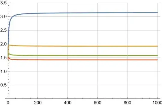
Below Python code computes an approximate value of $G(10^4)$ for $\alpha = \frac{1}{2}$ through Monte Carlo simulation using $10^6$ samples:

import numpy as np

def gen_sample(n): x = np.random.rand(n) ** (-2) return (np.sum(x) ** 2) / np.sum(x ** 2)

data = [gen_sample(10000) for _ in range(1000000)]

The exact value of lim G(n) is 3.188439615...

np.mean(data)

I got $3.1866881493312955$, which is reasonably close to the value $1+\frac{\Gamma (1/4)^2}{4 \Gamma (3/4)^2} = 3.188439615...$ we obtained from \eqref{main_res}.


Footnotes.

1) SLLN works whenever the expectation exists in the extended real number line $[-\infty, \infty]$.
Sangchul Lee
  • 181,930
  • Nice result for Pareto distribution. What about Pareto for $\alpha = 1$ as in comment? – River Li Nov 03 '23 at 07:38
  • 1
    @RiverLi, Thank you! When $\alpha = 1$, $G(n)$ diverges to $\infty$ at a speed of $(\log n)^2$ as in my heuristic computation. As for the proof strategy, only the estimate $(4)$ about the asymptotic behavior of $A_1(t)$ as $t \to 0^+$ needs modification. Then with the resulting modification of $(4)$ and mimicking my argument, we should be able to prove my previous comment. I decided not to include $\alpha=1$ case to my answer, though, because OP specifically requested examples for convergent $G(n)$, and more importantly, I'm exhausted now... :s – Sangchul Lee Nov 03 '23 at 07:46
  • For the SLLN to kick in for the sum of squares you need square integrability, $EX^2<\infty$. – Math-fun Nov 03 '23 at 07:49
  • 1
    @Math-fun, SLLN holds whenever the expectation exists in $[-\infty, \infty]$. In fact, the proof is quite easy assuming SLLN for the case of finite mean, using a truncation argument. See this for some famous references. :) – Sangchul Lee Nov 03 '23 at 07:52
  • Thanks a lot for the comment. For any iid random sequence $z_i$ you need the first moment to exist for the SLLN to go through for $\bar{z}$. For $X_i^2$ we hence need the second moment of $X_i$ to exist. :-) In your answer, you assume first moment to exist "only", yet use SLLN for $X_i^2$ (this was the point I wishes to clarify). – Math-fun Nov 03 '23 at 08:59
  • @SangchulLee Thanks. :) – River Li Nov 03 '23 at 09:09
  • 1
    @Math-fun, I guess you missed my point. SLLN actually works even when the expectation is either $+\infty$ or $-\infty$. (Hence, it only doesn't work when the expectation is undefined in $[-\infty,\infty]$.) Indeed, let $(X_i){i=1}^{\infty}$ be a sequence of i.i.d. random variables, sampled from the distribution of a r.v. $X$, such that either $\mathbf{E}[|X|]<\infty$, or $\mathbf{E}[X]=+\infty$, or $\mathbf{E}[X]=-\infty$. Then it follows that $$\lim{n\to\infty}\frac{X_1+\cdots+X_n}{n}=\mathbf{E}[X].$$ This is the version of SLLN I used in my answer and I mentioned in my previous comment. – Sangchul Lee Nov 03 '23 at 15:27
3

If the strong law of large numbers applies, then $$ \left(\frac{1}{n}\sum_{i=1}^n X_i\right)^2 \xrightarrow{\text{a.s.}} E[X]^2, \qquad \frac{1}{n}\sum_{i=1}^n {X_i}^2 \xrightarrow{\text{a.s.}} E[X^2].$$

Thus, $$ \frac{1}{n}\frac{\left(\sum X_i\right)^2}{\left(\sum {X_i}^2 \right)} = \frac{\left(\frac{1}{n}\sum X_i\right)^2}{\left(\frac{1}{n}\sum {X_i}^2 \right)} \xrightarrow{\text{a.s.}} \frac{E[X]^2}{E[X^2]}. $$

Therefore, if the strong law of large numbers applies for $\{X_i\}$ and $\{X_i^2\}$, then $$ \lim_{n\to\infty}\frac{G(n)}{n} = \frac{E[X]^2}{E[X^2]}.$$

From which we have that if $E[X]>0$, then $G(n) \to \infty$ as $n\to\infty$.

P.S. Dester
  • 1,157
  • 1
    As @Henry pointed out, OP is most likely wondering about for what $f$ is $\frac{1}{n}G(n)$ converging to a constant. And you showed that for at least all $f$ for which the SLLN applies, namely, at least all $f$ that have finite first moment. – William M. Aug 29 '23 at 17:45
  • @WilliamM. Apparently I was wrong about that. In any case you need a finite moment to say $\left(\frac{1}{n}\sum_{i=1}^n X_i\right)^2 \xrightarrow{\text{a.s.}} E[X]^2$ while the question does not suggest this – Henry Aug 29 '23 at 17:49
  • @WilliamM. It's amazing how you are the second person now to simply refuse to acknowledge that I meant to ask the question I asked. – XYZT Aug 29 '23 at 17:57
  • @XYZT if you only consider densities on $[0, 1],$ then this answers shows that "For no distribution (in this class) will $G(n)$ converge, and for all distributions (in this class) will $G(n) \sim c n,$ for a $c$ depending on the distribution." If this is not enough to what you are asking, then you probably don't know what you want to ask. If you allow for densities on $[0, \infty),$ then the problem is much harder. – William M. Aug 29 '23 at 18:02
  • If you bothered to read the question I posted, you would see that I did indeed say as much. "However, I suspect that it is not possible to get constant G at large-n for distributions on bounded intervals, anyway." Not only that, I literally provide a valid expression for the behavior of G(n) for distributions with finite moments. – XYZT Aug 29 '23 at 18:09
  • 1
    @XYZT, I have added an example when the LLT does not apply. – P.S. Dester Aug 29 '23 at 18:41
  • Also @XYZT, in my previous answer, I have provided sufficient conditions for which $G(n)$ diverges. I think that provides value to the post. I never said I had answered your question in totality, only for the cases in which LLT applies. Furthermore, that helped me to think about the example I provided. – P.S. Dester Aug 29 '23 at 18:44
  • Well, in the end, the example was not correct. I deleted it. – P.S. Dester Aug 29 '23 at 19:05
2

It does not answer the question, but too long for a comment.

Let $X_i$ follow a Pareto distribution of parameter $\alpha\in(0,1)$. Let $Y = \max\{X_1,\dots,X_n\}$. Using the law of total expectation, we can write that $$ G(n) = \mathbb{E}\!\left[\mathbb{E}\!\left[\frac{\left(\sum X_i\right)^2}{\left(\sum {X_i}^2 \right) } \mid Y \right]\right]. $$

For large $n$, we can say that $$ \mathbb{E}\!\left[\frac{\left(\sum X_i\right)^2}{\left(\sum {X_i}^2 \right) } \mid Y \right] \sim \frac{((n-1)E[X_1\mid Y] + Y)^2}{(n-1)E[X_1^2\mid Y] +Y^2 } = \frac{\left(\frac{\alpha (n-1) \left(Y-Y^{\alpha }\right)}{(1-\alpha ) \left(Y^{\alpha }-1\right)}+Y\right)^2}{\frac{\alpha (n-1) \left(Y^2-Y^{\alpha }\right)}{(2-\alpha) \left(Y^{\alpha }-1\right)}+Y^2} . $$

Then, we can calculate $G(n)$ using that $f_Y(y) = n \,\alpha\, y^{-\alpha -1} \left(1-y^{-\alpha }\right)^{n-1}$, $y>1$. But I couldn't do it analytically, so I plotted in Mathematica as a function of $n$ for $\alpha \in\{1/2,1/3,1/4,1/5\}$. G(n) as a function of <span class=$n$" />

Here is $G(n)$ as a function of $\alpha$ which is different from $(1-\alpha)^{-1}$: G(n) as a function of alpha

Here is the inverse of the expected value as a function of $\alpha$, which seems to agree with the $1-\alpha$ of Albrecher & Teugels (2007): Inverse as a function of alpha

P.S. Dester
  • 1,157
  • This might be a separate question in itself, but when do I know that the tail is heavy enough such that the maximum of $n$ random variables will dominate a sum of $n$ random variables? – user196574 Aug 30 '23 at 17:36
  • This certainly merits its own question. I imagine the necessary condition is that $E[X]$ does not exist. But I do not know if it is sufficient. – P.S. Dester Aug 30 '23 at 17:46
2

Let us denote $$\begin{align} &\bar{X}:=\frac{1}{n}\sum_{i=1}^nX_i\\ &\bar{X^2}:=\frac{1}{n}\sum_{i=1}^nX_i^2\\ \end{align}$$ then $$G(n,f) = n\cdot \mathbb{E}\left(\frac{(\bar{X})^2}{\bar{X^2}} \right)$$ According to the multidimensional central limit theorem:

$$ \begin{pmatrix} \bar{X}\\\bar{X^2} \end{pmatrix} \xrightarrow[\mathcal{D}]{n \to +\infty} \begin{pmatrix} \mathbb{E}(X)\\\mathbb{E}(X^2) \end{pmatrix} + \frac{1}{\sqrt{n}}\cdot\mathcal{N}_2\left( \begin{pmatrix} 0\\0 \end{pmatrix}; \begin{pmatrix} Var(X) & Cov(X,X^2)\\ Cov(X,X^2)& Var(X^2)\\ \end{pmatrix} \right) \tag{1} $$ We denote the gaussian vector $(Z,T)$ as follows $$\begin{pmatrix} Z\\T \end{pmatrix} := \mathcal{N}_2\left( \begin{pmatrix} 0\\0 \end{pmatrix}; \begin{pmatrix} Var(X) & Cov(X,X^2)\\ Cov(X,X^2)& Var(X^2)\\ \end{pmatrix} \right)$$ then from $(1)$

$$ G(n,f) \xrightarrow{n\to +\infty} n\cdot \mathbb{E} \left(\frac{\left(\mathbb{E}(X)+ \frac{1}{\sqrt{n}}Z \right)^2}{\mathbb{E}(X^2) + \frac{1}{\sqrt{n}}T} \right) \tag{2} $$

If $\mathbb{E}(X) \ne 0$, the numerator of $(2)$ converges to $\mathbb{E}^2(X)$ while the denumerator converges to $\mathbb{E}(X^2)$, the fraction inside the expectation converges to a positive value, then $G(n,f)$ must diverge.

So, we must have $$\mathbb{E}(X) = 0 \tag{3}$$

Applying $(3)$ to $(2)$, we have $$ \begin{align} G(n,f) \xrightarrow{n\to +\infty} n\cdot \mathbb{E} \left(\frac{\left( \frac{1}{\sqrt{n}}Z \right)^2}{\mathbb{E}(X^2) + \frac{1}{\sqrt{n}}T} \right) &=\mathbb{E} \left(\frac{Z^2}{\mathbb{E}(X^2) + \frac{1}{\sqrt{n}}T} \right) \\ &=\mathbb{E} \left(\frac{Z^2}{\mathbb{E}(X^2)} \cdot \frac{1}{1 + \frac{1}{\sqrt{n}} \frac{T}{\mathbb{E}(X^2)}} \right) \\ &\xrightarrow{n \to +\infty}\mathbb{E} \left(\frac{Z^2}{\mathbb{E}(X^2)} \right)\tag{4}\\ &=\frac{\mathbb{E}(Z^2)}{\mathbb{E}(X^2)} \\ & = \frac{Var(X)}{\mathbb{E}(X^2)} \\ & = \frac{\mathbb{E}(X^2) - \mathbb{E}^2(X)}{\mathbb{E}(X^2)} \\ & = 1 \end{align}$$

We conclude that $$ G(n,f) \xrightarrow{n\to +\infty} \begin{cases} +\infty &\text{if} \hspace{1cm} \mathbb{E}(X) \ne 0 \\ 1 &\text{if} \hspace{1cm} \mathbb{E}(X) = 0 \end{cases}\tag{5} $$ The result $(5)$ does not depend on the distribution of $X$ but depend on $\mathbb{E}(X)$.


I added the detail for $(4)$.

By using Taylor expansion, we have

$$\begin{align} L &:= \mathbb{E} \left(\frac{Z^2}{\mathbb{E}(X^2)} \cdot \frac{1}{1 + \frac{1}{\sqrt{n}} \frac{T}{\mathbb{E}(X^2)}} \right) \\ &=\mathbb{E} \left(\frac{Z^2}{\mathbb{E}(X^2)} \cdot \left(1+\sum_{i=1}^{+\infty} \frac{1}{n^{i/2}}\cdot \frac{T^{i}}{\mathbb{E}^{i}(X^2)} \right) \right)\\ &=\mathbb{E} \left(\frac{Z^2}{\mathbb{E}(X^2)} \right) + \sum_{i=1}^{+\infty} \frac{1}{n^{i/2}}\cdot \mathbb{E} \left(\frac{Z^2 T^{i}}{\mathbb{E}^{i}(X^2)} \right) \\ \end{align}$$

We observe that the variables $Z^2 T^{2k+1}$ are symetric in distribution and centered at $0$, so, $\mathbb{E}(Z^2 T^{i}) = 0$ for $i$ odd

Then $$\begin{align} L &= \mathbb{E} \left(\frac{Z^2}{\mathbb{E}(X^2)} \right) + \sum_{i=1}^{+\infty} \frac{1}{n^{i}}\cdot \mathbb{E} \left(\frac{Z^2 T^{2i}}{\mathbb{E}^{2i}(X^2)} \right) \\ &\le \mathbb{E} \left(\frac{Z^2}{\mathbb{E}(X^2)} \right) + \sum_{i=1}^{+\infty} \frac{1}{n^{i}}\cdot \frac{\sqrt{\mathbb{E}(Z^4)} \sqrt{ \mathbb{E}( T^{4i})}}{\mathbb{E}^{2i}(X^2)} \\ &\le \mathbb{E} \left(\frac{Z^2}{\mathbb{E}(X^2)} \right) + \sqrt{\mathbb{E}(Z^4)} \cdot \sum_{i=1}^{+\infty} \frac{1}{n^{i}}\cdot \frac{\sqrt{ \mathbb{E}( T^{4i})}}{\mathbb{E}^{2i}(X^2)} \tag{6} \end{align}$$

From the Jensen's inequality for the convex function $f(x):=x^i$ for $i\in \mathbb{N}$, we have: $$\mathbb{E}(T^{4i}) \le \mathbb{E}^i(T^{4})$$ then $$\begin{align} \mathbb{E} \left(\frac{Z^2}{\mathbb{E}(X^2)} \right) < L &\le \mathbb{E} \left(\frac{Z^2}{\mathbb{E}(X^2)} \right) + \sqrt{\mathbb{E}(Z^4)} \cdot \sum_{i=1}^{+\infty} \left(\frac{1}{n}\cdot \frac{\mathbb{E}^{1/2}(T^4)}{\mathbb{E}^2(X^2)} \right)^i \\ &=\mathbb{E} \left(\frac{Z^2}{\mathbb{E}(X^2)} \right) + \underbrace{ \frac{1}{n}\cdot \frac{\mathbb{E}^{1/2}(T^4)}{\mathbb{E}^2(X^2)} \cdot \frac{1}{1-\frac{1}{n}\cdot \frac{\mathbb{E}^{1/2}(T^4)}{\mathbb{E}^2(X^2)}}}_\text{converge to $0$ when $n \to +\infty$} \end{align}$$

Then $$G(n,f) \xrightarrow{n\to +\infty} \frac{\mathbb{E}(Z^2)}{\mathbb{E}(X^2)}$$

NN2
  • 20,162
  • 1
    Hello @NN2, just a quick question: how can we justify that convergence in distribution implies convergence of expectations here? Some uniform integrability argument? – Snoop Aug 30 '23 at 08:10
  • @Snoop Thank for your remark, I just added the detail for $(4)$ in the end of the answer. – NN2 Aug 30 '23 at 10:04
  • 1
    @NN2 +1 This is nice, but I worry it hits many of the same points as the other answers. Namely, when the CLT applies, or when the SLLN applies, then one gets $$G(n,f) \xrightarrow{n\to +\infty} \begin{cases} +\infty &\text{if} \hspace{1cm} \mathbb{E}(X) \ne 0 \ 1 &\text{if} \hspace{1cm} \mathbb{E}(X) = 0 \end{cases}$$ In particular, these assumptions hold trivially when the support of the random variable is on $[0,1]$.

    The more challenging aspect of this question is the case of support on $[0,\infty]$, specifically cases when the moments of $X$ do not exist.

    – user196574 Aug 30 '23 at 17:43
2

Some thoughts.

For some distributions, e.g. uniform distribution, we can obtain the asymptotic expressions in the following way.

Using the identity ($q > 0$) $$ \frac{1}{q} = \int_0^\infty \mathrm{e}^{-qt}\,\mathrm{d} t, $$ letting $f_k(t) := \mathbb{E}\left(X_1^k\mathrm{e}^{-t X_1^2}\right)$ for $k = 0, 1, 2, \cdots$, using IBP, we have \begin{align*} &\mathbb{E}\left[\frac{(\sum_i X_i)^2}{\sum_i X_i^2}\right]\\[6pt] ={}& 1 + \mathbb{E}\left[\frac{\sum_{1\le i< j \le n} 2X_iX_j}{\sum_i X_i^2}\right]\\[6pt] ={}& 1 + \mathbb{E}\left[\left(\sum_{1\le i< j\le n} 2X_iX_j\right) \cdot \int_0^\infty \mathrm{e}^{-t\sum_i X_i^2}\,\mathrm{d} t\right]\\[6pt] ={}& 1 + n(n-1)\int_0^\infty \left[\mathbb{E}\left(X_1 \mathrm{e}^{-t X_1^2}\right)\right]^2\left[\mathbb{E}\left(\mathrm{e}^{-t X_1^2}\right)\right]^{n-2}\,\mathrm{d} t\\[6pt] ={}& 1 + n(n-1)\int_0^\infty [f_1(t)]^2[f_0(t)]^{n-2}\,\mathrm{d} t\\[6pt] ={}& 1 - n\int_0^\infty \frac{[f_1(t)]^2}{f_2(t)}\,\mathrm{d} [f_0(t)]^{n-1} \tag{1}\\[6pt] ={}& 1 + n\cdot \lim_{t\to 0^{+}} \frac{[f_1(t)]^2}{f_2(t)} + n\int_0^\infty [f_0(t)]^{n-1}\cdot \frac{-2f_1(t)f_3(t)f_2(t) + [f_1(t)]^2f_4(t)}{[f_2(t)]^2}\,\mathrm{d} t \tag{2}. \end{align*} Explanation:
(1): Use $f_0'(t) = f_2(t)$.
(2): Use $\lim_{t\to 0^{+}} f_0(t) = 1$, and $\lim_{t\to \infty} \frac{[f_1(t)]^2}{f_2(t)}[f_0(t)]^{n-1} = 0$ using $f_0(t)f_2(t) \ge [f_1(t)]^2$ for all $t \ge 0$ (C-S inequality) and $\lim_{t\to \infty} f_0(t) = 0$.

$\phantom{2}$

  • Ex. 1: Uniform distribution $X_1 \sim U(0, 1)$

Using IBP for (2), we have \begin{align*} &\mathbb{E}\left[\frac{(\sum_i X_i)^2}{\sum_i X_i^2}\right]\\[6pt] ={}& 1 + n\cdot \lim_{t\to 0^{+}} \frac{[f_1(t)]^2}{f_2(t)} - \int_0^\infty \frac{-2f_1(t)f_3(t)f_2(t) + [f_1(t)]^2f_4(t)}{[f_2(t)]^3}\,\mathrm{d} [f_0(t)]^n\\[6pt] ={}& 1 + n\cdot \lim_{t\to 0^{+}} \frac{[f_1(t)]^2}{f_2(t)} + \lim_{t\to 0^{+}} \frac{-2f_1(t)f_3(t)f_2(t) + [f_1(t)]^2f_4(t)}{[f_2(t)]^3} \\[6pt] &\qquad + \int_0^\infty [f_0(t)]^n \cdot \left(\frac{-2f_1(t)f_3(t)f_2(t) + [f_1(t)]^2f_4(t)}{[f_2(t)]^3}\right)'\,\mathrm{d} t \end{align*} which gives $$G(n; U(0, 1)) = \frac34 n + \frac{1}{10} + o(1).$$ Explanation:

(i): $\lim_{t\to 0^{+}} \frac{[f_1(t)]^2}{f_2(t)} = \frac{\left[\mathbb{E}\left(X_1 \right)\right]^2}{\mathbb{E}\left(X_1^2\right)} = \frac34$.

(ii): $\lim_{t\to 0^{+}} \frac{-2f_1(t)f_3(t)f_2(t) + [f_1(t)]^2f_4(t)}{[f_2(t)]^3} = \frac{-2\mathbb{E}\left(X_1\right)\mathbb{E}\left(X_1^3\right)\mathbb{E}\left(X_1^2\right) + [\mathbb{E}\left(X_1\right)]^2\mathbb{E}\left(X_1^4\right)}{[\mathbb{E}\left(X_1^2\right)]^3} = - \frac{9}{10}$.

(iii): $|(\frac{-2f_1(t)f_3(t)f_2(t) + [f_1(t)]^2f_4(t)}{[f_2(t)]^3})'|$ is bounded by constant $C$. We have $|\int_0^\infty [f_0(t)]^n \cdot (\frac{-2f_1(t)f_3(t)f_2(t) + [f_1(t)]^2f_4(t)}{[f_2(t)]^3})'\,\mathrm{d} t| \le C \int_0^\infty [f_0(t)]^n\, \mathrm{d} t = o(1)$.

$\phantom{2}$

  • Ex. 2: Pareto distribution $X_1 = \frac{1}{x^2}{\bf 1}_{x > 1}$

We have $\lim_{t\to 0^{+}} \frac{[f_1(t)]^2}{f_2(t)} = 0$. We have \begin{align*} &\mathbb{E}\left[\frac{(\sum_i X_i)^2}{\sum_i X_i^2}\right]\\[6pt] ={}& 1 + n\int_0^\infty [f_0(t)]^{n-1}\cdot \frac{-2f_1(t)f_3(t)f_2(t) + [f_1(t)]^2f_4(t)}{[f_2(t)]^2}\,\mathrm{d} t. \end{align*} (Note: $\mathbb{E}(X_1) = \infty$ and $\mathbb{E}(X_1^2) = \infty$.)

To be continued.

River Li
  • 49,125
  • 2
    Nice observation! Following this idea and assuming $f_{X_i}(x) = \frac{1}{x^2}\mathbf{1}{{x>1}}$ is the Pareto distribution, then my back-of-the-envelope computation gives $$G(n) \approx 1 + \int{0}^{\infty}e^{-\sqrt{\pi x}}\left(\log n - \frac{\log s + \gamma}{2}\right)^2 , \mathrm{d}s. $$ – Sangchul Lee Nov 02 '23 at 07:59
  • @SangchulLee Thanks. Your expression is nice. Did you deal with something like my last expression (Ex. 2) in the new version? – River Li Nov 02 '23 at 14:03
  • 1
    I started from the representation $$G(n)=1 + n(n-1)\int_{0}^{\infty} f_0(t)^{n-2} f_1(t)^2 ,\mathrm{d}t$$ and then utilized various asymptotic formulas for $f_0$ and $f_1$. Take my claim with a grain of salt, though, because my computation is only heuristic. (Of course, I believe it can be improved to a rigorous proof, and Monte-Carlo simulation up to $n=102400$ shows that the above formula works well.) – Sangchul Lee Nov 02 '23 at 20:55
  • @SangchulLee Very nice. – River Li Nov 02 '23 at 22:47