Understanding Karush-Kuhn-Tucker conditions

Question

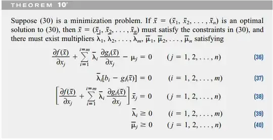
Suppose we may want to use the K–T conditions to find the optimal solution to: \begin{array}{cc} \max & (\text { or } \min ) z=f\left(x_{1}, x_{2}, \ldots, x_{n}\right) \\ \text { s.t. } & g_{1}\left(x_{1}, x_{2}, \ldots, x_{n}\right) \leq b_{1} \\ & g_{2}\left(x_{1}, x_{2}, \ldots, x_{n}\right) \leq b_{2} \\ & \vdots \\ &g_{m}\left(x_{1}, x_{2}, \ldots, x_{n}\right) \leq b_{m} \\ & -x_{1} \leq 0 \\ & -x_{2} \leq 0 \\ & \vdots \\ & -x_{n} \leq 0 \end{array} then the theorem state the KT condition as:

Which I really don't understand and eventually failed to applied as my book didn't illustrate any example with details. For sake of clarity, let's pick one minimization problem,

\begin{array}{ll} \text { Minimize } & Z=2 x_{1}+3 x_{2}-x_{1}^{2}-2 x_{2}^{2} \\ \text { subject to } & x_{1}+3 x_{2} \leq 6 \\ & 5 x_{1}+2 x_{2} \leq 10 \\ & x_{1} \geq 0, i=1,2 . \end{array}

After google searching and watching YouTube video, I find they solve it by,

$$L(x_1,x_2,x_3,\lambda_1,\lambda_2)=2 x_{1}+3 x_{2}-x_{1}^{2}-2 x_{2}^{2}+\lambda_1(x_{1}+3 x_{2}-6)+\lambda_2(5 x_{1}+2 x_{2}-10)$$

$(1)$ Assuming both $g_1$ and $g_2$ active:

Solving $\frac{\partial L}{\partial x_1}=0,\frac{\partial L}{\partial x_2}=0,\frac{\partial L}{\partial \lambda_1}=0,\frac{\partial L}{\partial \lambda_2}=0 \implies \left(\frac{18}{13},\frac{20}{13},\frac{185}{169},-\frac{11}{169}\right)$ Which can't accept.

$(2)$ Assuming $g_1$ active:

Solving $\frac{\partial L}{\partial x_1}=0,\frac{\partial L}{\partial x_2}=0,\frac{\partial L}{\partial \lambda_1}=0 \implies \left(\frac{3}{2},\frac{3}{2},1,0\right)$, hence $z=\frac34$

$(3)$ Assuming $g_2$ active:

Solving $\frac{\partial L}{\partial x_1}=0,\frac{\partial L}{\partial x_2}=0,\frac{\partial L}{\partial \lambda_2}=0 \implies \left(\frac{89}{54},\frac{95}{108},0,\frac{7}{27}\right)$, hence $z=\frac{371}{216}$

$(4)$ Assume none of constraint is active:

Solving $\frac{\partial L}{\partial x_1}=0,\frac{\partial L}{\partial x_2}=0 \implies \left(1,\frac{3}{4}\right)$ hence $z=\frac{17}{8}$

Hence, $z_{\min}=\frac{3}{4}$

---

So, I was confusing how the second method satisfy the theorem $10$? Like did they do the same thing? Checking the inequality is binding or not? And could I write the second method on exam as a solution for KKT condition?

Answer 1

First try to understand the following simplified version of KKT:

Suppose you are trying to solve the problem

$$\text{min } f(x)$$

$$\text{s.t. } g_j(x) \leq b_j$$

Where (if i don't recall bad, $f$ and the $g_i$ are convex). Then KKT conditions tell you that if $x^*$ is a solution then you can find $\lambda_j$ such that:

1. $\lambda_j \geq 0$ for all $j$
2. $\lambda_j [g_j(x^*)-b_j]=0$ for all $j$
3. $\frac{\partial f}{\partial x_i}(x^*)+ \sum_j \lambda_j \frac{\partial g_j}{\partial x_i}(x^*)=0$ for all $i$ or equivalently $\nabla f + \sum_j \lambda_j \nabla g_j=0$

Note that the sets $g_j(x)=b_j$ form the boundary of your domain. Look at condition 2. It basically says: "either $x^*$ is in the part of the boundary given by $g_j(x^*)=b_j$ or $\lambda_j=0$. When $g_j(x^*)=b_j$ it is said that $g_j$ is active. So in this setting, the general strategy is to go through each constraint and consider wether it is active or not.

As you can see, condition 2. is independent of $f$, it is just about the location of $x^*$ in the domain. It is about "how many constraints does $x^*$ hit sharply"? Note that for example if no $g_j$ is active, then $\lambda_j=0$ for all $j$ and you are looking for solutions to $\frac{\partial f}{\partial x_i}(x^*)=0$ ie extreme points of $f$.

Now suppose there is only one constraint, call it $g$, and suppose it is active. The you have something like this situation:

(Sorry for handwritten picture but I am so bad at drawing with the computer)

So if $x^*$ is a minimum of $f$ then it means that when you take points $x'$ inside the domain $A$, $f(x')$ is greater than $f(x^*)$. Now, since $g$ is convex, the vector $-\nabla g$ does always point inwards (or paralell), so you would like $f$ to increase in the direction of $\nabla g$. This applies to all points of the border of the boundary $g(x)=0$ so one would think that a minimum must be one where $f$ increases "the most" in the direction of $\nabla g$. Since the direction in which $f$ increases is given by its gradient, you want $\nabla f(x^*)$ and $-\nabla g (x^*)$ to be proportional one to another by a ppositive constant. This exaclty means that there exists some $\lambda \geq 0$ such that $\nabla f = - \lambda \nabla g$. These are precisely conditions 3. and 1., and this reasoning generalizes to more constraints.

(Note that here I am explaining things vaguely. the fact that this works uses strongly that $f$ and $g$ are convex and is precisely is the statement of the Theorem of KKT, whcih is not trivial)

Now, how does this translate to your example? In your example you have two type of restrictions: given by some unknown funtions $g_j$ and other ones given by $-x_i \leq 0$. Let's apply the conditions 1.-3. to the problem $$\text{min } f(x)$$

$$\text{s.t. } g_j(x) \leq b_j \quad\text{and}\quad -x_j\leq 0 $$

Let's call $h_i$ the function sending $x$ to $-x_i$. We should have multipliers $\lambda_j$ (corresponding to the $g_j$) and $\mu_i$ (corresponding to the constraints $h_i \leq 0$) such that

• (1)$\lambda_j, \mu_i \geq 0$ for all $i,j$.
• (2a) $\lambda_j (g_j(x^*)-b_j)=0$ for all $j$.
• (2b) $\mu_i(h_i(x^*)-0)=0$ or equivalently $\mu_i x_i=0$ for all $i$.
• (3) $\nabla f(x^*) + \sum_j \lambda_j \nabla g(x^*) + \sum_i \mu_i \nabla h_i(x^*)=0$.

But $\nabla h_i = (0,\ldots , -1, \ldots 0)$ so the conditions in (3) actually read as

$$\frac{\partial f}{\partial x_i}(x^*)+ \sum_j \lambda_j \frac{\partial g_j}{\partial x_i}(x^*) - \mu_i=0$$

Therefore, regarding your text, (39) and (40) is just (1), (36) is (3), (37) is (2a) and (38) is (2b) after sustitution of $\mu_i = \frac{\partial f}{\partial x_i}(x^*)+ \sum_j \lambda_j \frac{\partial g_j}{\partial x_i}(x^*)$ into the equation $x_i \mu_i=0$.

The 'method for solving these problems' given in the Youtube video is just setting the conditions to be active or not, which is the same as doing: if $\lambda_j (g_j(x^*)-b_j)=0$ then either $\lambda_j=0$ of $g_i(x^*)=b_j$, except that you don't do the ones for the constraints $\mu_ix_i=0$ because they are easy to handle without making new cases, since you would have to condider $2^4=16$ possibilities...

Answer 2

[This is a very heuristic explanation of KKT conditions.]

Ref: “Foundations of Applied Mathematics, Vol 2” by Humpherys, Jarvis.

Consider the optimization problem

$${ {\begin{align} &\, \text{minimize } \quad f(x) \\ &\, \text{subject to } \quad G(x) \preceq 0, \, \, H(x) = 0 \end{align}} }$$

where ${ f : \mathbb{R} ^n \longrightarrow \mathbb{R} }$ and ${ G : \mathbb{R} ^n \longrightarrow \mathbb{R} ^m, }$ ${ H : \mathbb{R} ^n \longrightarrow \mathbb{R} ^{\ell} }$ are smooth functions.

Let ${ x ^{\ast} }$ be a local minimizer of ${ f(x) }$ under the constraints ${ G(x) \preceq 0, }$ ${ H(x) = 0 . }$

What are the conditions which ${ x ^{\ast} }$ must satisfy?

For any feasible point ${ x \in \mathscr{F} }$ we can consider the index set of binding constraints

$${ J(x) := \lbrace j : g _j (x) = 0 \rbrace }$$

and the locus of binding constraints

$${ \widetilde{\mathscr{F}}(x) := \lbrace y : H(y) = 0, \, \, g _j (y) = 0 \text{ for all } j \in J(x) \rbrace . }$$

Note that locally near ${ x ^{\ast} , }$ the nonbinding constraints

$${ g _j (y) < 0, \quad \text{ for all } \, \, j \in [m] \setminus J(x ^{\ast}) }$$

are automatically satisfied.

Hence we can focus on ${ \widetilde{\mathscr{F}}(x ^{\ast}) , }$ and the fact that ${ x ^{\ast} }$ is a local minimizer of ${ f }$ over ${ \widetilde{\mathscr{F}}(x ^{\ast}) . }$

Thm [KKT conditions]
Suppose the local minimizer ${ x ^{\ast} }$ is also a regular point of ${ \widetilde{\mathscr{F}}(x ^{\ast}) . }$ That is, the collection of gradients

$${ (\nabla h _i (x ^{\ast})) _{i=1} ^{\ell}, \quad (\nabla g _j (x ^{\ast})) _{j \in J(x ^{\ast})} }$$

are linearly independent. (Note that this is generically true).
Then there exist ${ \lambda ^{\ast} \in \mathbb{R} ^{\ell} , }$ ${ \mu ^{\ast} \in \mathbb{R} ^m }$ such that

• ${ Df(x ^{\ast}) + (\lambda ^{\ast}) ^{T} DH(x ^{\ast}) + (\mu ^{\ast}) ^T DG(x ^{\ast}) = 0. }$

• ${ \mu ^{\ast} \succeq 0 . }$

• ${ \mu _j ^{\ast} g _j (x ^{\ast}) = 0 }$ for all ${ j \in [m] . }$

Pf: Note that ${ x ^{\ast} }$ is a local minimizer of ${ f }$ over ${ \widetilde{\mathscr{F}}(x ^{\ast}) . }$ Note that ${ x ^{\ast} }$ is a regular point of ${ \widetilde{\mathscr{F}}(x ^{\ast}) . }$ Hence by classical Lagrange multipliers, there exist ${ \lambda ^{\ast} \in \mathbb{R} ^{\ell} }$ and ${ (\mu _j ^{\ast}) _{j \in J(x ^{\ast})} }$ such that

$${ D f(x ^{\ast}) + \sum _{i = 1} ^{\ell} \lambda _i ^{\ast} D h _i (x ^{\ast}) + \sum _{j \in J(x ^{\ast})} \mu _j ^{\ast} D g _j (x ^{\ast}) = 0 . }$$

Define ${ \mu _j ^{\ast} := 0 }$ for ${ j \in [m] \setminus J(x ^{\ast}) . }$ Note that this gives a vector ${ \mu ^{\ast} \in \mathbb{R} ^m . }$

Note that by definition ${ \mu _j ^{\ast} = 0 }$ for ${ j \in [m] \setminus J(x ^{\ast}) ,}$ and ${ g _j (x ^{\ast}) = 0 }$ for ${ j \in J (x ^{\ast}) . }$ Hence

$${ \mu _j ^{\ast} g _j (x ^{\ast}) = 0 \quad \text{ for all } j \in [m] . }$$

Note that

$${ Df(x ^{\ast}) + (\lambda ^{\ast}) ^{T} DH(x ^{\ast}) + (\mu ^{\ast}) ^T DG(x ^{\ast}) = 0 . }$$

Hence it suffices to show

$${ \text{To show: } \quad \mu ^{\ast} \succeq 0 . }$$

Let ${ k \in J(x ^{\ast}) . }$ It suffices to show

$${ \text{To show: } \quad \mu ^{\ast} _k \geq 0 . }$$

Suppose to the contrary ${ \mu ^{\ast} _k < 0 . }$ Consider ${ \widetilde{\mathscr{F}}(x ^{\ast}) _k , }$ the enlargement of ${ \widetilde{\mathscr{F}}(x ^{\ast}) }$ on removing the ${ g _k = 0 }$ constraint.

Note that the normal space

$${ T _{x ^{\ast}} \widetilde{\mathscr{F}}(x ^{\ast}) _k ^{\perp} = \text{span}\left( (\nabla h _i (x ^{\ast})) _{i=1} ^{\ell}, (\nabla g _j (x ^{\ast})) _{j \in J(x ^{\ast}) \setminus \lbrace k \rbrace } \right) . }$$

Hence

$${ \nabla g _k (x ^{\ast}) \not\in T _{x ^{\ast}} \widetilde{\mathscr{F}}(x ^{\ast}) _k ^{\perp} . }$$

Hence there is a direction ${ v }$ such that

$${ v \in T _{x ^{\ast}} \widetilde{\mathscr{F}}(x ^{\ast}) _k , \quad \langle \nabla g _k (x ^{\ast}), v \rangle < 0 . }$$

Note that

$${ {\begin{aligned} &\, \langle \nabla f (x ^{\ast}), v \rangle \\ = &\, - \sum _{i=1} ^{\ell} \lambda _i ^{\ast} \langle \nabla h _i (x ^{\ast}) , v \rangle - \sum _{j = 1} ^{m} \mu _j ^{\ast} \langle \nabla g _j (x ^{\ast}), v \rangle \\ = &\, - \mu _k ^{\ast} \langle \nabla g _k (x ^{\ast}), v \rangle . \end{aligned}} }$$

Hence the direction ${ v }$ satisfies

$${ v \in T _{x ^{\ast}} \widetilde{\mathscr{F}}(x ^{\ast}) _k , \quad \langle \nabla g _k (x ^{\ast}), v \rangle < 0, \quad \langle \nabla f (x ^{\ast}), v \rangle < 0 . }$$

Hence, if we perturb ${ x ^{\ast} }$ in the direction ${ v , }$ we will approximately stay in ${ \widetilde{\mathscr{F}}(x ^{\ast}) _k \cap \lbrace g _k < 0 \rbrace }$ and ${ f }$ decreases.

Hence, if we perturb ${ x ^{\ast} }$ in the direction ${ v , }$ we will approximately stay in ${ \mathscr{F} }$ and ${ f }$ decreases. A contradiction.

Hence ${ \mu _k ^{\ast} \geq 0, }$ as needed. ${ \blacksquare }$