1

I want to learn how to use the Karush-Kuhn-Tucker (KKT) conditions to solve a quadratic programming problem with both equality and in-equality constraints.

The problem in question is set in finance and it consists in finding the best constantly re-balanced portfolio in hindsight, i.e. a portfolio that maximizes the logarithmic wealth in hindsight. In other words, given a matrix of multivariate returns $ \left( R_{i,t} \right)_{i,t=1,1}^{N,T} $we are looking for a vector $ {\bf b} := \left( b_i \right)_{i=1}^N $ such that :

\begin{equation} {\bf b}^{*} = \mbox{argmax}_{{\bf b}} \sum\limits_{\xi=1}^T \log(1 + {\bf b} \cdot \vec{R}_\xi ) \tag{1} \end{equation}

subject to the following constraints:

  1. No leverage: $ |{\bf b}| = b_1+b_2+ \cdots + b_N = 1$,
  2. No short selling: $ b_i \ge 0 $ for $i=1,\cdots, N$.
Note 1:

In practice, problem $(1)$ can be formulated as a quadratic minimization problem. In fact by expanding the logarithm in a series to the second order we need to solve the following:

\begin{equation} {\bf b}^{*} = \mbox{argmin}_{{\bf b}} \sum\limits_{\xi=1}^T \left( - {\bf b} \cdot \vec{\mu} + \frac{1}{2} {\bf b}^{T} \cdot {\bf c} \cdot {\bf b} \tag{2} \right) \end{equation}

where $ \vec{\mu} = \left( \mu_i\right)_{i=1}^N $ where $\mu_i = \sum\limits_{\xi=1}^T R_{i,\xi} $ for $i=1,\cdots,N$ and ${\bf c}:= \left( c_{i,j} \right)_{i,j=1}^N$ where $ c_{i,j} := \sum\limits_{\xi=1}^T R_{i,\xi} R_{j,\xi} $ for $i,j,=1,\cdots,N $.

Note 2:

The solution to the unconstrained problem, i.e. with the constraints 2. being waived, reads:

\begin{equation} {\bar {\bf b}}^{*} = {\bf c}^{-1} \cdot \left( \vec{\mu} - \lambda 1_{N \times 1}\right) \tag{3} \end{equation}

where $1_{N \times 1}$ is a column vector of length $N$ composed of ones and the constant $\lambda $ satisfies the following equation $1_{N,1}^{T} \cdot {\bf c}^{-1} \left( \vec{\mu} - \lambda \right) = 1 $.


Now, I have followed the Numerical Example in here to code the KKT conditions. In short what I do is the following. I start with the solution $(3)$ and then find which in-equality constraints (no short-selling) are violated. Then I make those constraints active, i.e. I add those constraints to the the Lagrange function. In other words my new Lagrange function reads:

\begin{equation} L\left( {\bf b}; {\bf \kappa}, \lambda \right) := - {\bf b} \cdot \vec{\mu} + \frac{1}{2} {\bf b}^{T} \cdot {\bf c} \cdot {\bf b} + \sum\limits_{j=1, j\in {\mathfrak J}}^{N} \kappa_j \cdot (-b_j) + \lambda \left( \left| {\bf b} \right| - 1 \right) \tag{4} \end{equation}

where ${\mathfrak J} := \left( j \in \left\{1,\cdots, N \right\} | b^{*}_j < 0 \right) = \left( \eta_1,\eta_2, \cdots, \eta_m\right) $ and $ {\bar {\bf b}}^{*} := \left( b^{*}_j\right)_{j=1}^N $.

Now, by taking the gradient of $(4)$ by the allocation vector and setting it to zero we get:

\begin{eqnarray} \frac{\partial }{\partial b_i} L\left( {\bf b}; {\bf \kappa}, \lambda \right) = - \mu_i + \sum\limits_{j=1}^N {\bf c}_{i,j} {\bf b}_j + \sum\limits_{j=1, j\in {\mathfrak J}}^{N} \kappa_j \cdot (-\delta_{j,i}) + \lambda &=& 0 & \quad \mbox{for $i=1,\cdots,N$} \tag{5a} \\ b_j &=& 0 & \quad \mbox{for $j \in {\mathfrak J}$} \tag{5b} \\ b_1+b_2 + \cdots b_{N} &=& 1 \tag{5c} \end{eqnarray} where $m := card({\mathfrak J}) $.

The equations $(5a)-(5c)$ constitute a system of $N + m$ linear equations with unknowns $\vec{r}:= \left(b_1,b_2,\cdots,b_N;\kappa_{\eta_1},\cdots,\kappa_{\eta_m}; \lambda\right)$. I solve the aforementioned equations by solving a following system of linear equations:

\begin{equation} \left( \begin{array}{lll} {\bf c} & - {\bf m}_{1,2} & {\bf 1}_{N,1} \\ -{\bf m}_{1,2}^{T} & {\bf 0}_{m,m} & {\bf 0}_{m,1} \\ {\bf 1}_{1,N} & {\bf 0}_{1,m} & {\bf 0}_{1,1} \end{array} \right) \cdot \vec{r} = \left( \begin{array}{l} \vec{\mu} \\ {\bf 0}_{m,1} \\ 1 \end{array} \right) \tag{6} \end{equation}

where $ {\bf m}_{1,2} := \left( \delta_{\eta_j, i} \right)_{i=1,j=1}^{N,m} $

I have written a simple program in Matlab that codes equations $(6)$ as below.

%This is to test the quadratic programming algo with both equality and
%in-equality constraints as formulated in the Example in
%https://optimization.cbe.cornell.edu/index.php?title=Quadratic_programming.
close all;
%%%%%%%%%%%%%%%%%%%%%%%%%%%%%%%%%%
% Generate the time series.
%%%%%%%%%%%%%%%%%%%%%%%%%%%%%%%%%%
tmp = rand(1,6); [r1,r2,r3,z12,z13,z23]=deal(tmp(1),tmp(2),tmp(3),tmp(4),tmp(5),tmp(6));
%Number of assets and the length of time series.
dim  = randi([10,20],1);p1 = randi([1,dim-2],1);p2 = randi([p1+1,dim-1],1);T = 1000;dt= 1/256;
% The underlying correlation matrix and the drifts,
Sigma = ConstructBlockDiagonalMatrix([r1 z12 z13; z12 r2 z23; z13 z23 r3],[p1, p2-p1 dim-p2]);
mu = rand(dim,1)/256;
R=  randn(dim,T);
% The prices S, the returns R and the price relatives X.
S = cumprod(1 + mu*dt + Sigma*sqrt(dt)*R,2);
R = diff(S,1,2)./S(:,1:end-1);
X = S(:,2:end)./S(:,1:end-1);
figure; semilogy(S');xlabel('time');ylabel('prices');

%An approximate closed form expression for bstar. %Old way. [rhs,mat] = deal(zeros(dim-1,1),zeros(dim-1)); for xi=1:dim-1 rhs(xi) = sum((R(xi,:) - R(xi+1,:)) ./ (1+R(dim,:))); for eta=1:dim-1 mat(xi,eta) = sum((R(xi,:) - R(xi+1,:)) .* (R(eta,:) - R(eta+1,:)) ./ (1+R(dim,:)).^2); end end bstarApr = mat \ rhs; bstarApr =[bstarApr(1) diff(bstarApr)' 1-bstarApr(end)]'; %New way. [rhs,mat] = deal(zeros(dim,1),zeros(dim)); for xi=1:dim rhs(xi) = sum(R(xi,:)); for eta=1:dim mat(xi,eta) = sum( R(xi,:) .* R(eta,:) ); end end mones = ones(1,dim); lmb= ( mones (mat \ rhs) - 1 )/( mones (mat \ mones') ); bstarApr1 = mat \ (rhs - lmb * ones(dim,1)); bstarApr2=quadprog(mat,-rhs,[],[],ones(1,dim),1);

%Solve the constrained problem by using the Karush-Kuhn-Tucker theorem https://en.wikipedia.org/wiki/Karush-Kuhn-Tucker_conditions %See also example from https://optimization.cbe.cornell.edu/index.php?title=Quadratic_programming Theta1 = find(bstarApr1 < 0); dim1 = length(Theta1); mat12 = -cell2mat(arrayfun(@(xi) (xi == Theta1), 1:dim, 'UniformOutput', false))'; Mat = ... { mat, mat12, ones(dim,1); ... -mat12', zeros(dim1,dim1), zeros(dim1,1); ... ones(1,dim), zeros(1,dim1), zeros(1,1)}; Mat=cell2mat(Mat); % Sanity check: % 2x1 & 3x1 block: all(arrayfun(@(xi) Mat(dim+xi,Theta1(xi)),1:dim1 )==1) all(Mat(dim+dim1+1,1:dim)==1) % 1x2 block: all(arrayfun(@(p) Mat(Theta1(p),dim+p),1:dim1)==-1) Rhs={rhs; zeros(dim1,1); ones(1)}; Rhs= cell2mat(Rhs);%Rhs(end)=[]; Vars = Mat \ Rhs; [Mu1] = deal(Vars(dim+(1:dim1))); %Drop constraints for which Mu's are negative. Theta1new = Theta1; Theta1new(Mu1 <0 )=[]; bstarConstr=quadprog(mat,-rhs,-eye(dim),zeros(1,dim),ones(1,dim),1); disp('bstar unconstr. ours | bstar unconstr. quadprog | bstar constr ours | bstar constr. quadprog()'); [bstarApr1, bstarApr2, Vars(1:dim) bstarConstr]

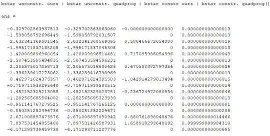
This program outputs the un-constrained solution $(3)$ along with the output of Matlab's quadprog() routine (the first two columns on the left) and the constrained solution along with the respective quadprog output (last two columns on the right).

enter image description here

As you can see the first two columns match (as they should) but the last two columns don't.

In view of that I have two following questions.

The first question is what it is that I am doing wrong in the calculations above?

The second question is how would you be using the KKT conditions to solve the Markowitz portfolio optimization problem, i.e. to maximize the mean return of the portfolio subject to a given variance (volatility) and subject to all the asset allocations being non-negative (long only).
RobPratt
  • 50,938
Przemo
  • 11,971
  • 1
  • 25
  • 56
  • Many optimization algorithms can be interpreted as solving the KKT conditions (using an iterative method), but except in special cases it is usually not possible to write down the KKT conditions on paper and solve analytically. So what you need is just an appropriate optimization algorithm. One choice that would be fairly easy to implement from scratch is the proximal gradient method, or an accelerated proximal gradient method such as FISTA. Boyd’s manuscript on proximal algorithms is one place to learn more about that. Vandenberghe’s UCLA 236c notes are also very good. – littleO Aug 10 '23 at 09:31

2 Answers2

1

This is an answer to the first question.

There is a very nice detailed explanation of how KKT conditions work in the first answer to this question. The most important thing is to find the right number of constraints in $(5b)$ that are active, meaning such constraints that turn the in-equalities into equalities at the optimal solution. That set of active constraints is definitely somewhere between ${\mathfrak J}$ (the set of constraints being violated in ${\bar {\bf b}^{*} }$) and $\left\{1,\cdots, N \right\}$ (the set of all constraints). Having this in mind one strategy is to start from the minimal set, meaning ${\mathfrak J}$, and then basing on the output components that are non-positive add additional constraints until the set in question does not change anymore. Having tested this on my system and I conclude that this algorithm converges in most cases after no more than four loop passes and the answer does not differ from the output of Matlab's quadprog() routine. The new code looks as follows.

%This is to test the quadratic programming algo with both equality and
%in-equality constraints as formulated in the Example in
%https://optimization.cbe.cornell.edu/index.php?title=Quadratic_programming.
close all;
%%%%%%%%%%%%%%%%%%%%%%%%%%%%%%%%%%
% Generate the time series.
%%%%%%%%%%%%%%%%%%%%%%%%%%%%%%%%%%
tmp = rand(1,6); [r1,r2,r3,z12,z13,z23]=deal(tmp(1),tmp(2),tmp(3),tmp(4),tmp(5),tmp(6));
%Number of assets and the length of time series.
dim  = randi([10,20],1);p1 = randi([1,dim-2],1);p2 = randi([p1+1,dim-1],1);T = 1000;dt= 1/256;
% The underlying correlation matrix and the drifts,
Sigma = ConstructBlockDiagonalMatrix([r1 z12 z13; z12 r2 z23; z13 z23 r3],[p1, p2-p1 dim-p2]);
mu = rand(dim,1)/256;
R=  randn(dim,T);
% The prices S, the returns R and the price relatives X.
S = cumprod(1 + mu*dt + Sigma*sqrt(dt)*R,2);
R = diff(S,1,2)./S(:,1:end-1);
X = S(:,2:end)./S(:,1:end-1);
figure; semilogy(S');xlabel('time');ylabel('prices');

%An approximate closed form expression for bstar. %Old way. [rhs,mat] = deal(zeros(dim-1,1),zeros(dim-1)); for xi=1:dim-1 rhs(xi) = sum((R(xi,:) - R(xi+1,:)) ./ (1+R(dim,:))); for eta=1:dim-1 mat(xi,eta) = sum((R(xi,:) - R(xi+1,:)) .* (R(eta,:) - R(eta+1,:)) ./ (1+R(dim,:)).^2); end end bstarApr = mat \ rhs; bstarApr =[bstarApr(1) diff(bstarApr)' 1-bstarApr(end)]'; %New way. [rhs,mat] = deal(zeros(dim,1),zeros(dim)); for xi=1:dim rhs(xi) = sum(R(xi,:)); for eta=1:dim mat(xi,eta) = sum( R(xi,:) .* R(eta,:) ); end end mones = ones(1,dim); lmb= ( mones (mat \ rhs) - 1 )/( mones (mat \ mones') ); bstarApr1 = mat \ (rhs - lmb * ones(dim,1)); bstarApr2=quadprog(mat,-rhs,[],[],ones(1,dim),1);

%Solve the constrained problem by using the Karush-Kuhn-Tucker theorem https://en.wikipedia.org/wiki/Karush-Kuhn-Tucker_conditions %See also example from https://optimization.cbe.cornell.edu/index.php?title=Quadratic_programming [count,Theta1] = deal(0,find(bstarApr1 < 0)); while 1 dim1 = length(Theta1); mat12 = -cell2mat(arrayfun(@(xi) (xi == Theta1), 1:dim, 'UniformOutput', false))'; Mat = ... { mat, mat12, ones(dim,1); ... -mat12', zeros(dim1,dim1), zeros(dim1,1); ... ones(1,dim), zeros(1,dim1), zeros(1,1)}; Mat=cell2mat(Mat); % Sanity check: % 2x1 & 3x1 block: all(arrayfun(@(xi) Mat(dim+xi,Theta1(xi)),1:dim1 )==1) all(Mat(dim+dim1+1,1:dim)==1) % 1x2 block: all(arrayfun(@(p) Mat(Theta1(p),dim+p),1:dim1)==-1) Rhs={rhs; zeros(dim1,1); ones(1)}; Rhs= cell2mat(Rhs);%Rhs(end)=[]; Vars = Mat \ Rhs; [bstarC,Mu1] = deal(Vars(1:dim),Vars(dim+(1:dim1))); bstarConstr=quadprog(mat,-rhs,-eye(dim),zeros(1,dim),ones(1,dim),1); makenewconstrsactive = find(bstarC<0); disp('bstar unconstr. ours | bstar unconstr. quadprog | bstar constr ours | bstar constr. quadprog()'); disp([bstarApr1, bstarApr2, bstarC, bstarConstr]); Theta1new = unique([Theta1; makenewconstrsactive]); if size(Theta1new) == size(Theta1), break; else, Theta1 = Theta1new; end count = count + 1; %input('Press any key when ready.'); end disp(['Algorithm converged after ' num2str(count) ' loop passes.']);

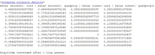
And the output is below:

enter image description here

As we can see now both the first two left-most and the first two right-most columns match.

Przemo
  • 11,971
  • 1
  • 25
  • 56
0

This is an answer to the second question. In the Markowitz optimization we assume that the financial time series are described by a multivariate Gaussian with known (and time independent) vector of mean returns $\vec{\mu}$ and a covariance matrix ${\bf C} $. As such the objective function (for the unconstrained problem) reads:

\begin{equation} L(\vec{\omega};\lambda) := - \vec{\omega}^{T} \cdot \vec{\mu} + \lambda \cdot \left( \vec{\omega}^{T} \cdot {\bf C} \cdot \vec{\omega} - \sigma^2\right) \tag{1} \end{equation}

Here $\vec{\omega} := \left( \omega_i \right)_{i=1}^N$ are the asset allocations, $\sigma^2$ is the variance of the portfolio (the target volatility) and $\lambda$ is the Lagrange multiplier. Now, by setting the partial derivatives with respect to the allocations and the Lagrange multiplier to zero we obtain the following (unconstrained) solution:

\begin{equation} \vec{\omega}^{*} = \sigma \cdot \frac{{\bf C}^{-1} \cdot \vec{\mu}}{\sqrt{\vec{\mu}^{T} \cdot {\bf C}^{-1} \cdot \vec{\mu} }} \tag{1a} \end{equation}

Now, clearly in the solution $(1a)$ some of the asset allocations will be negative, i.e. some of the constraints will be violated. By denote by ${\mathfrak J} := \left( (j_\xi )_{\xi=1}^m | 1 \le j_\xi \le N \right) $ the (distinct) indices of the constraints being violated. Now we modify the objective function in question by adding the new constraints. We have:

\begin{equation} L(\vec{\omega}; \vec{\kappa},\lambda) = - \vec{\omega}^{T} \cdot \vec{\mu} + \lambda \cdot \left( \vec{\omega}^{T} \cdot {\bf C} \cdot \vec{\omega} - \sigma^2\right) + \sum\limits_{\xi=1}^m (- \omega_{j_\xi} ) \cdot \kappa_{j_\xi} \tag{2} \end{equation}

Now the vector of unknowns is the following $\left( \omega_1,\cdots,\omega_N; \kappa_{j_1}, \cdots, \kappa_{j_m}; \lambda \right)$. We differentiate the objective function $(2)$ by those unknowns (from the left to the right) and get the following equations:

\begin{eqnarray} - \mu_i + 2 \lambda \left({\bf C} \vec{\omega} \right)_{i} + \sum\limits_{\xi=1}^m \kappa_{j_\xi} \cdot (-\delta_{j_\xi,i}) &=&0 & \quad \mbox{for $i=1,\cdots,N$} \\ - \omega_{j_\xi} &=& 0 & \quad \mbox{for $\xi=1,\cdots,m$} \\ \vec{\omega}^{T} \cdot {\bf C} \cdot \vec{\omega} &=& \sigma^2 \tag{3} \end{eqnarray}

The first $N+m$ equations in $(3)$ are linear so they can be written in a matrix form as follows:

\begin{equation} \left( \begin{array}{lll} 2 \lambda \cdot {\bf C}_{N,N} & {\bf B}_{N,m} \\ {\bf B}^{T}_{m,N} & {\bf 0}_{m,m} \end{array} \right) \cdot \left( \begin{array}{l} \omega_1 \\ \vdots \\ \omega_N \\ \kappa_{j_1} \\ \vdots \\ \kappa_{j_m} \end{array} \right) = \left( \begin{array}{l} \mu_1 \\ \vdots \\ \mu_N \\ 0 \\ \vdots \\ 0 \end{array} \right) \tag{4} \end{equation} where ${\bf B}_{N,m} := \left( - \delta_{j_\xi,i} \right)_{i=1,\xi=1}^{N,m}$.

By using block matrix inversion we obtain a following closed form solution of the system $(4)$. We have:

\begin{eqnarray} \left( \begin{array}{l} \omega_1 \\ \vdots \\ \omega_N \end{array} \right) &=& \frac{1}{2 \lambda} {\bf C}^{-1} \underbrace{\left[ 1 - {\bf B} \left( {\bf B}^T \cdot {\bf C}^{-1} \cdot {\bf B} \right)^{-1} \cdot {\bf B}^{T} {\bf C}^{-1}\right] }_{{\bf \Upsilon}}\cdot \left( \begin{array}{l} \mu_1 \\ \vdots \\ \mu_N \end{array} \right) \tag{5a} \\ % \left( \begin{array}{l} \kappa_{j_1} \\ \vdots \\ \kappa_{j_m} \end{array} \right) &=& \left( {\bf B}^{T} {\bf C}^{-1} {\bf B} \right)^{-1} \cdot {\bf B}^{T} {\bf C}^{-1} \cdot \left( \begin{array}{l} \mu_1 \\ \vdots \\ \mu_N \end{array} \right) \tag{5b} \end{eqnarray}

Now, inserting $(5a)$ into the last equation in $(3)$ gives us a following closed form solution for the weights:

\begin{equation} \vec{\omega}^{**} := \sigma \cdot \frac{{\bf C}^{-1} \cdot {\bf \Upsilon} \cdot \vec{\mu}}{\sqrt{\vec{\mu}^{T} \cdot {\bf \Upsilon}^{T} \cdot {\bf C}^{-1} \cdot {\bf \Upsilon} \cdot \vec{\mu} }} \tag{6} \end{equation}

As we can see the solution $(6)$ is the same as the familiar old one $(1a)$ except that $\vec{\mu}$ is being replaced by ${\bf \Upsilon} \cdot \vec{\mu}$. Here the solution $(6)$ has to be computed iteratively starting from the unconstrained one and then by adding new constraints to the set ${\mathfrak J}$ until the set does not change anymore.


Now we have tested the solution $(6)$ . We generated a bunch of random walks with different drift values and a certain covariance matrix. We took a set of target volatilities $\sigma_0 = linspace( 0.1, 0.2, 10)$. For each target volatility we plot the asset allocations for both KKT (top) and Matlab's fmincon routine (bottom). Here the different target volatilities correspond to different colors (from blue to red respectively). In addition to that , for each target volatility, I also check if all the constraints are satisfied -- see text output on the very left. Here you go:

close all;
% % Load the price returns A(:,:)
% load(['C:\Users\PRepetowicz\Documents\Coras\temp\matfiles' filesep 'AforPR.mat']);
% R = A;%returns.
% A = cumprod(1+R,2);%prices

%%%%%%%%%%%%%%%%%%%%%%%%%%%%%%%%%% % Generate the time series. %%%%%%%%%%%%%%%%%%%%%%%%%%%%%%%%%% tmp = rand(1,6); [r1,r2,r3,z12,z13,z23]=deal(tmp(1),tmp(2),tmp(3),tmp(4),tmp(5),tmp(6)); %Number of assets and the length of time series. dim = randi([10,20],1);p1 = randi([1,dim-2],1);p2 = randi([p1+1,dim-1],1);T = 1000;dt= 1/256; % The underlying correlation matrix and the drifts, Sigma = ConstructBlockDiagonalMatrix([r1 z12 z13; z12 r2 z23; z13 z23 r3],[p1, p2-p1 dim-p2]); mu = 0.9rand(dim,1)/256; sigma0 = sqrt(0.1rand()/256); R= randn(dim,T); % The prices A, the returns R and the price relatives X. A = cumprod(1 + mudt + sigma0Sigmasqrt(dt)R,2); R = diff(A,1,2)./A(:,1:end-1); X = A(:,2:end)./A(:,1:end-1); cols = jet(size(A,1)); h=figure(1); myh=semilogy(A');set(myh,{'Color'}, num2cell(cols, 2));xlabel('time');ylabel('prices');title('Underlying assets'); hold on;

num=10; mytargetvols = linspace(0.1, 0.2,num);

C=cov(R'); mu=mean(R,2); n = length(mu);

[which,myws,mywws] = deal(1,zeros(num,n),zeros(num,n));

for s00=mytargetvols s0=s00/sqrt(252);

% The unconstrained solution.
w=C\(mu);
imask = find( w &lt; 0 );
m=length(imask);count=0;

while true
    % size(B) is n x m
    B = -cell2mat(arrayfun(@(xi) (xi == imask), 1:n, 'UniformOutput', false))';

    % Compute the inverse of a block matrix as in https://en.wikipedia.org/wiki/Block_matrix
    tmp = B' * (C \ B);
    sqBrckt = ( eye(n ) - B * ( tmp \ (C \ B)') );

    if sum(sum(abs(sqBrckt))) &lt; 1e-10, w = zeros(n,1); k = mu; break; end

    % Normalization
    Nrm = sqrt( (sqBrckt * mu)' * (C \ sqBrckt) * mu );

    % The weights size = n x 1
    w = s0/Nrm *( C \ sqBrckt) * mu;
    % The additional Lagrange multipliers size = m x 1
    k =  (tmp  \ (C \ B)') * mu;

    imasknew = unique( [imask'  find( w &lt; 0 )'])';
    if sum(imasknew) == sum(imask), break; end
    %input(['Press any key when ready. imask=' num2str(imask')]);
    imask = imasknew;
    count = count + 1;
end
disp(['KKT conditions converged in ' num2str(count) ' loop passes.']);
% Verify conditions.
condts= [abs(sum(w(imask).* k)) &lt; 1e-10, abs(w' * C * w - s0^2) &lt; 1e-10, all(w &gt; -1e-10)];
disp(['vec(w)^T * vec(k) eq. zero, vol eq. s0^2, w &gt;0: ' num2str(condts)]);


options = optimoptions('fmincon','Algorithm','interior-point','Display','off'); % run interior-point algorithm
options.MaxFunctionEvaluations = 10000;
[ww, fval]= fmincon(@(w) - w'* mu,1/n*ones(n,1),-eye(n),zeros(n,1),[],[],[],[],@(w) mycon(w,s0,C),options);


myws (which,:) = w';
mywws(which,:) = ww';
which=which+1;

end cols = jet(num); figure(2); subplot(2,1,1);myh=plot(myws'); set(myh,{'Color'}, num2cell(cols, 2));xlabel('assets');ylabel('allocations');title('KKT conditions'); subplot(2,1,2);myh=plot(mywws'); set(myh,{'Color'}, num2cell(cols, 2));xlabel('assets');ylabel('allocations');title('fmincon');

figure(1);myh=semilogy(cumprod(1 + ww' * R));myh.Marker = '*';myh.Color=[0 0 0];

function [c,ceq] = mycon(w,s0,C) c = []; ceq = w' * C *w - s0^2; end

enter image description here

As you can see the KKT conditions lead to exactly the same result as the output of the black-box routine fmincon. For some reasons all the allocations end up being concentrated on few assets only . It would be good to understand the mechanism for this phenomenon.

Note 1:

There are some exceptional cases when KKT and fmincon() lead to different results. Note that the crucial quantity in the algorithm above is the set of active constraints ${\mathfrak J}$.

That set is initialized to constraints being violated in the un-constrained solution, i.e. ${\mathfrak J} := \left\{ 1 \le j \le N | \omega^{*}_j < 0 \right \}$ and then after each loop pass it is amalgamated with the indices of updated solution where the constraints are still violated, i.e. ${\mathfrak J} = {\mathfrak J} \cup ( \vec{\omega}_{new}^{*} <0 )$. This is being done until the set in question does not change any more and reaches some final value ${\bar {\mathfrak J}}$. Now most of the time that final value is different from the set of all constraints $\left\{ 1,2,\cdots, N\right\}$ but in some rare cases it may happen otherwise. In that case the matrix ${\bf \Upsilon} = {\bf 0}$ and then the optimal allocations being returned by KKT are all equal to zero. This is what happened in the case below. Here the number of assets was $N=10$. Here we go:

enter image description here

As you can see out of the three conditions the second one, i.e. of the volatility hitting the target, is not satisfied for obvious reasons-- all allocations are zero. More importantly though fmincon() gives a different answer. The conclusion from that is that in those rare cases the scheme above does not give us the optimal solution.

Przemo
  • 11,971
  • 1
  • 25
  • 56