25

Usually, the use of matrix multiplication is initially given with graphics — scalings, translations, rotations, etc. Then, there are more in-depth examples such as counting the number of walks between nodes in a graph using the power of the graph's adjacency matrix.

What are other good examples of using matrix multiplication in various contexts?

Vass
  • 1,543
  • Edited tags to remove "examples" and add "big-list", which this question promises to become. This probably also should be community-wiki. – Niel de Beaudrap May 27 '11 at 20:12
  • Isn't this question equivalent to "What are good examples of compositions of finite-dimensional linear operators in various contexts?" –  May 28 '11 at 03:44
  • 4
    No, matrices and finite-dimensional linear operators are not the same. They are the same only after choosing a basis, which is an important distinction. – the L May 28 '11 at 07:25

8 Answers8

10

Linear discrete dynamical systems, aka recurrence relations, are best studied in a matrix formulation $x_{n+1} = A x_n$. The solution of course is $x_n = A^n x_0$, but the point is to exploit the properties of $A$ to allow the computation of $A^n$ without performing all multiplications. As an example, take the Fibonacci numbers. The formula for them comes directly from this matrix formulation (plus diagonalization).

Don't forget the origins of matrix multiplication: linear change of coordinates. See, for instance, section 3.4 of Meyers's book (page 93) at http://web.archive.org/web/20110714050059/matrixanalysis.com/Chapter3.pdf.

See also http://en.wikipedia.org/wiki/Matrix_multiplication#Application_Example.

u243676
  • 115
  • 5
lhf
  • 221,500
10

A fundamental example is the multivariate chain rule. A basic principle in mathematics is that if a problem is hard, you should try to linearize it so that you can reduce as much of it as possible to linear algebra. Often this means replacing a function with a linear approximation (its Jacobian), and then composition of functions becomes multiplication of Jacobians. But of course there are many other ways to reduce a problem to linear algebra.

Qiaochu Yuan
  • 468,795
8

Matrix multiplcation plays an important role in quantum mechanics, and all throughout physics. Examples include the moment of inertia tensor, continuous-time descriptions of the evolution of physical systems using Hamiltonians (especially in systems with a finite number of basis states), and the most general formulation of the Lorentz transformation from special relativity.

General relativity also makes use of tensors, which are a generalization of the sorts of objects which row-vectors, column-vectors, and matrices all are. Very roughly speaking, row- and column-vectors are 'one dimensional' tensors, having only one index for its coefficients, and matrices are 'two dimensional' tensors, having two indices for its coefficients, of two different 'kinds' representing rows and columns — input and output, if you prefer. Tensors allow three or more indices, and to allow more than one index to have the same 'kind'.

  • I don't understand what you mean by row and column indices being comparable to "input" and "output". – Brennan Vincent May 29 '11 at 07:37
  • Consider the convention (common in physics) of representing vectors by columns. We then often identify linear transformations T : ℝⁿ¹ → ℝⁿ² using a matrix of dimensions n₂×n₁ matrix: multiplying such a matrix T by a column-vector x ∈ ℝⁿ¹ yields another column vector T x ∈ ℝⁿ². The column space of T defines the output, and the row-space defines the input. Furthermore, fixing a column index 'a' of T (identifying a single column) determines the output given the standard basis vector eₐ as input; the row-index then describes the coefficients of the vector which is output. – Niel de Beaudrap May 29 '11 at 08:59
7

Matrix multiplication — more specifically, powers of a given matrix A — are a useful tool in graph theory, where the matrix in question is the adjacency matrix of a graph or a directed graph.

More generally, one can interpret matrices as representing (possibly weighted) edges in a directed graph which may or may not have loops, and products of matrices as specifying the total number (or total weight) of all the walks with a given structure, between pairs of vertices.

  • 1
    Floyd-Warshall algorithm for finding all pair shortest-path in a weighted graph can be viewed as computing powers of the adjacency matrix of the graph, where the multiplication $A^2 = A \otimes A$ is defined over the semiring $(\mathbb{R}, min, +, \infty).$ –  May 28 '11 at 00:48
  • +1! I came across this result in some papers of Janzing and Wocjan on BQP-complete problems on mixing times for large graphs. That work at least partly motivated a question on the HHL algorithm with ${0,1}$ entries, that you helped me formalize a couple of years ago. – Mark S May 13 '23 at 15:07
  • Misha Lavrov dug up some of the history on the relationship between powers and the number of walks. – Mark S May 13 '23 at 15:07
6

Matrices are heavily used in mathematical finance in various ways. One specific example is a correlation matrix where an entry (i,j) specifies the degree to which price movements in instrument i and instrument j are correlated over a specified time period. A huge number of computer cycles is spent daily on computing these sorts of matrices and applying further analysis to them in order to, in part, attempt to quantify the amount of risk associated with a portfolio of instruments.

ItsNotObvious
  • 11,263
6

Hey Alex, a central theme of Machine Learning is about finding structures (preferably linear ones) in the data space; the intrinsic dimentionalities of your observations if you may (see Eigenfaces).

I understand this may not be about matrix multiplication per se; instead, this is about what, many times, happens right before it. It begins with the spectral theorem: A = SΛS' (inverse when A is non-symmetric); it is Literally the basis of so many things (see what I did there?).

5

High-dimensional problems in statistical physics can sometimes be solved directly using matrix multiplication, see http://en.wikipedia.org/wiki/Transfer_matrix_method. The best-known example of this trick is the one-dimensional Ising model http://en.wikipedia.org/wiki/Ising_model, where an $N$-particle system can be 'solved' by calculating the $N$-th power of a 2x2-matrix, which is (almost) trivial; otherwise, one would have to compute a sum over $2^N$ terms to get the same result.

Gerben
  • 806
1

1) Matrix multiplication is the majority of deep learning and convolutional neural networks

In case you were under a rock, from 2012 on onwards deep learning algorithms have quickly become the best known algorithms for a variety of problems, including notably image classification, in which convolutional neural network (CNN) are used (deep learning with some convolution layers), and notably running on GPUs as opposed to CPUs.

And deep learning and convolutional neural networks are to a large extent (dense) matrix multiplication, both in the training and inference phases. This article explains it well: https://petewarden.com/2015/04/20/why-gemm-is-at-the-heart-of-deep-learning/ Basically two key stages can be reduced to matrix multiplications:

  • fully connected layers
  • convolution

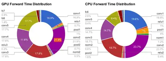
Benchmarks from this 2014 thesis by Yangqing Jia: https://www2.eecs.berkeley.edu/Pubs/TechRpts/2014/EECS-2014-93.pdf showing that:

  • convolution (convX operations like conv1, conv2, etc.) make up basically the entire runtime of ImageNet's Krizhevsky et al. (AKA AlexNet)
  • fcX are fully connected layers. Here we see that they don't take up much time, possibly because the previous convolutional layers have already reduced the original image size by a lot

enter image description here

Fully connected layers

Fully connected layers look like this: https://www.researchgate.net/profile/Adhistya-Permanasari-2/publication/265784353/figure/fig1/AS:669201052209156@1536561372912/Architecture-of-Multi-Layer-Perceptron-MLP.png

enter image description here

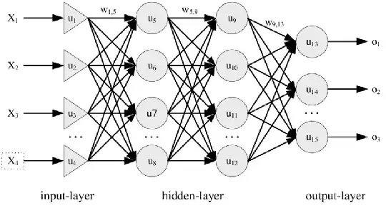
Each arrow has a weight. The computation of the activation for layer is very directly a matrix-vector multiplication, where:

  • inputs: vector with activation from previous layer
  • matrix: contains the weights
  • outputs: vector with activation for the next layer (to be followed by activation function)

We cannot further paralelize this as actual matrix-matrix multiplication however, it has to happen in sequence, because the value of one layer depends on the previous one being fully computed.

Convolution layers

Convolution layers can actually be converted to matrix-matrix multipliation as shown at https://petewarden.com/2015/04/20/why-gemm-is-at-the-heart-of-deep-learning/ section "How GEMM works for Convolutions":

enter image description here

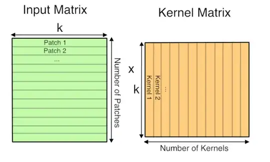
It may require some memory copying to put things in the right format however, which is a shame, but likely generally worth it, related: https://stackoverflow.com/questions/868568/what-do-the-terms-cpu-bound-and-i-o-bound-mean/33510470#33510470

Well explained at: https://www.youtube.com/watch?v=aircAruvnKk But what is a neural network? | Chapter 1, Deep learning by 3Blue1Brown (2017)

2) 3D rendering applications

Some ideas at: https://computergraphics.stackexchange.com/questions/8704/why-does-opengl-use-4d-matrices-for-everything/13324#13324

3) Quantum computing

I guess this is directly linked to more general uses of matrix multiplication in quantum mechanics in general. But at least this use case is more specific and digestible for my brain.

In order to evaluate the output of a quantum circuit, we can first convert it to a matrix, which can be done deterministically.

Given an input, the probability of each output of a quantum circuit is found by doing matrix multiplication with that matrix.

Suppose we have a 3 qubit system. The inputs could be one of eight.

000
001
010
011
100
101
110
111

Given N qubits, the circuit matrix is $2^n \times 2^n$. For each input, we map it to a vector of size $2^N = 2^3 = 8$ as follows:

000 -> 1000 0000 == (1.0, 0.0, 0.0, 0.0,  0.0, 0.0, 0.0, 0.0)
001 -> 0100 0000 == (0.0, 1.0, 0.0, 0.0,  0.0, 0.0, 0.0, 0.0)
010 -> 0010 0000 == (0.0, 0.0, 1.0, 0.0,  0.0, 0.0, 0.0, 0.0)
011 -> 0001 0000 == (0.0, 0.0, 0.0, 1.0,  0.0, 0.0, 0.0, 0.0)
100 -> 0000 1000 == (0.0, 0.0, 0.0, 0.0,  1.0, 0.0, 0.0, 0.0)
101 -> 0000 0100 == (0.0, 0.0, 0.0, 0.0,  0.0, 1.0, 0.0, 0.0)
110 -> 0000 0010 == (0.0, 0.0, 0.0, 0.0,  0.0, 0.0, 1.0, 0.0)
111 -> 0000 0001 == (0.0, 0.0, 0.0, 0.0,  0.0, 0.0, 0.0, 1.0)

The output of a 3 qubit circuit is necessarily 3 bits.

To obtain the probability of each output after an experiment, we simply multiply the 8-vectors by the 8x8 matrix.

Suppose that the result of this multiplication for the input 000 is:

$$ \begin{aligned} \vec{q_{out}} &= \begin{bmatrix} \frac{\sqrt{3}}{2} \\ 0.0 \\ \frac{1}{2} \\ 0.0 \\ 0.0 \\ 0.0 \\ 0.0 \\ 0.0 \end{bmatrix} \end{aligned} $$

Then, the probability of each possible outcomes would be the length of each component squared:

$$ \begin{aligned} P(000) &= \left|\frac{\sqrt{3}}{2}\right|^2 &= \frac{\sqrt{3}}{2}^2 &= \frac{3}{4} \\ P(001) &= \left|0\right|^2 &= 0^2 &= 0 \\ P(010) &= \left|\frac{\sqrt{1}}{2}\right|^2 &= \frac{\sqrt{1}}{2}^2 &= \frac{1}{4} \\ P(011) &= \left|0\right|^2 &= 0^2 &= 0 \\ P(100) &= \left|0\right|^2 &= 0^2 &= 0 \\ P(101) &= \left|0\right|^2 &= 0^2 &= 0 \\ P(110) &= \left|0\right|^2 &= 0^2 &= 0 \\ P(111) &= \left|0\right|^2 &= 0^2 &= 0 \\ \end{aligned} $$

so in this case, 000 would be the most likely outcome, with 3/4 probability, followed by 010 with 1/4 probability, all other outputs being impossible.

Therefore, if 000 is the correct output for input 000, then we can reach arbitrary confidence that the result is correct by running the experiment over and over.