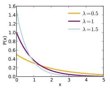
One issue is that, unlike probability, probability density is dimensionful—it is probability per unit of some quantity, where that quantity may have units. Changing measurement units will therefore change the probability density. So if $f$ is the pdf for the distribution of heights of adult males, measured in meters, and you suddenly decide to measure heights in centimeters, the corresponding probability density will be $100$ times smaller. This ensures that the probability that height is between $1.6$ m and $1.9$ m is the same as the probability that the height is between $160$ cm and $190$ cm. Specifically, if $g$ is the pdf for heights measured in centimeters, then $g(100x)=0.01\cdot f(x)$, and
$$
\int_{160}^{190}g(y)\,dy=\int_{1.6}^{1.9}g(100x)\cdot100\,dx=\int_{1.6}^{1.9}f(x)\,dx.
$$
An implication of this is that, by choosing measurement units suitably, you can make probability density have any numerical value you want (including values bigger than $1$).
Because of this dependence on units, probability density is not so fundamental. But that doesn't mean it is meaningless. For example, $f(1.6)$ is approximately the probability that height lies within a one meter interval around $1.6$ m, say $P(1.1\le x\le 2.1)$, while $g(160)$ is approximately the probability that height lies within a one centimeter interval around $160$ cm, say $P(159.5\le y\le 160.5)$. Clearly $g(160)$ is going to be a more reasonable approximation of the quantity it represents than is $f(1.6)$ since the pdf is much closer to being constant between $159.5$ cm and $160.5$ cm than it is between $1.1$ m and $2.1$ m.
The main point is that, in a density function, it is area, not height, that represents probability. The value of $f$ is the height; integrals of $f$ are areas. Values $f(x)$ are useful insofar as they allow you to compute areas. The interpretations of $f(1.6)$ and $g(160)$ in the previous paragraph are based on approximating areas by rectangles (of unit width).
Your relative probability interpretation is basically correct. Your statement that $p(1)/p(0)=4.67$ means that $x=1$ is $4.67$ as likely as $x=0$ would be more correctly stated as $P(1-\epsilon/2\le x\le1+\epsilon/2)$ is approximately $4.67$ times as big is $P(-\epsilon/2\le x\le\epsilon/2)$, or even more correctly as
$$
\lim_{\epsilon\to0}\frac{P(1-\epsilon/2\le x\le1+\epsilon/2)}{P(-\epsilon/2\le x\le\epsilon/2)}=4.67.
$$
In fact, $P(x=1)$ and $P(x=0)$ are both $0$: for a continuous quantity, the probability that $x$ equals a particular value, to infinite precision, is $0$.
The best way to gain intuition for the pdf is to practice making histograms, which is something you do in a descriptive statistics course. This will give you a feeling for why it is best that area represent probability, and not height. The idea is that, by choosing area, the height and shape of the histogram are relatively insensitive to the choice of bin width, and even to varying the bin widths within a single histogram. For example, if there are $1000$ data points, and $100$ of them lie between $1.6$ m and $1.8$ m then, if heights were used to represent probability, that bin would be a rectangle of width $0.2$ m and height $\frac{100}{1000}=0.1$. Now suppose that $55$ of the data points lay between $1.6$ and $1.7$ and $45$ between $1.7$ and $1.8$. Rebinning would produce two rectangles of width $0.1$ m and heights $0.055$ and $0.045$, which are roughly half the previous height. With areas used to represent probability, the first histogram would have a bin of width $0.2$ m and height $\frac{0.1}{0.2}=0.5\ \mathrm{m}^{-1}$, and the second would have two rectangles of widths $0.1$ m and heights $\frac{0.55}{0.1}=0.55\ \mathrm{m}^{-1}$ and $\frac{0.45}{0.1}=0.45\ \mathrm{m}^{-1}$, which are very close to the original height. By doing things using the area method, you avoid having to change (and reinterpret) your vertical scale every time you change bin size.
