2

I'm supposed to generate random numbers from the following distribution:

$$ f(x) = \begin{cases} \frac{3}{4}(2x-x^2) &\mbox{if } x \in (0,2) \\ 0 & \mbox{else} \end{cases} $$

I'm given the following algorithm in my script, which looks slightly different from those that I have found in the literature:

  1. Simulate $ U \sim U(0,1)$
  2. Simulate $Y \sim q$
  3. Accept $X=Y$ if $ U \leq \dfrac{1}{M}\dfrac{f(Y)}{q(Y)}$, otherwise go to step 1.

Now first I have to find a function q which is easier to sample from, such that there exists a $M \in \mathbb{R}$, so that $Mq(x) \geq f(x), \forall x \in (0,2)$.

I decided to pick $q \sim U(0,2)$ and have $M := \sup_{x \in (0,2)} f(x) = \frac{3}{4}$

Now I sample from $U(0,1)$, for which I get $U = 0.32$, then I sample from $Y \sim q \Rightarrow 1.28$ and now I'm supposed to accept the sampled value $y$ from step 2 if $ U \leq \frac{1}{M} \frac{f(Y)}{q(Y)}$ which in my case gives me: $0.32 \leq \frac{4}{3}f(1.29)=0.92$, so I'm supposed to accept $X=1.28$, however $1.28$ can hardly be from $f$. So what am I doing wrong.

eager2learn
  • 2,839
  • 1
    Why can't $X=1.28$ be from $f$? I think it can. The support of $f$ is $(0,2)$ and $x=1.28$ is in this interval. – Jimmy R. Jan 23 '16 at 15:12
  • Oh, and what is this $g$ in the denominator? Should it be $q$? – Jimmy R. Jan 23 '16 at 15:15
  • 1
    What you're doing should work: you are essentially sampling uniformly from the rectangle $[0,2] \times [0,3/4]$, which contains the entire graph of your PDF, and then accepting the $x$ value of any points that lie under the graph of your PDF. Visually it should be clear why this makes sense. – Ian Jan 23 '16 at 15:16
  • @JimmyR. Doesn't X have to be an element from the range of f? Maybe I'm totally confused right now, but isn't the point of this to sample values from the density f? E.g. if I sample from a standard normal distribution, I wouldn't expect a very large value to be sampled, even though that value is part of the domain of the standard normal. – eager2learn Jan 23 '16 at 15:30
  • @eager2learn Yes, your intuition is correct. And $x=1.28$ is almost directly in the middle of the domain of $f$, so why does it bother you? – Jimmy R. Jan 23 '16 at 15:56
  • What I don't really understand is how 1.28 can be drawn from f when f has a maximum value of 0.75 on the interval (0,2). I just don't see why we should sample values from the domain of f and not the range. – eager2learn Jan 23 '16 at 16:13
  • 2
    @eager2learn The value of a PDF at a given point essentially tells you how likely that point is to appear in a sample. (It's not actually a probability, but still, this is the rough idea.) So we are always sampling from the domain of the PDF. Proceeding otherwise would create a ton of problems: for one thing, we would never be able to sample negative numbers. – Ian Jan 23 '16 at 16:20
  • ah yes, that was kind of stupid on my part. Thanks for clearing that up. – eager2learn Jan 23 '16 at 16:24

1 Answers1

2

I think part of your original confusion is that your 'envelope' function is too simple. Let's start (as in the crucial comment by @Ian) 
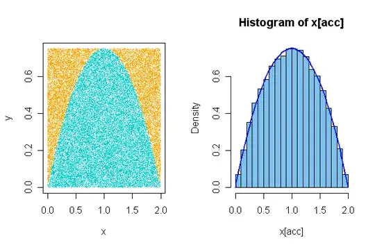
by generating points uniformly in the rectangle that encloses your PDF $f(x) = 0.75(2x - x^2),$ for $x \in [0,2].$ Points (blue) that fall under the PDF curve are accepted and those above it (orange) are rejected. A histogram of the accepted x-values fits the PDF well. You can verify by integration that the simulated values of $E(X)$ and $SD(X)$ are correct within simulation error. (My R code below, saves all points and then settles which ones are accepted at the end.)

 B = 40000;  M = 3/4
 x = runif(B, 0, 2);  y = runif(B, 0, M)
 acc = y <= M*(2*x - x^2)
 mean(x[acc]);  sd(x[acc])
 ## 1.002849  # Simulated E(X)
 ## 0.446792  # Simulated SD(X)

 par(mfrow = c(1,2))  # side-by-side plots
   plot(x, y, pch=".", col="red")
     points(x[acc], y[acc], pch=".")
   hist(x[acc], prob=T, col="wheat")
     curve(.75*(2*x - x^2), 0, 2, lwd=2, col="blue", add=T)
 par(mfrow = c(1,1))  # restore default plotting

enter image description here

In practice, it often 'wastes' too many candidate values to simulate within a rectangle, so an 'envelope' function is chosen for the upper boundary. In your more general notation, the envelope function is $M$ times the density function of $Unif(0, 2)$. It may help you to remember how this method works if you rewrite my code in your more general notation.

Notes: (a) Your PDF is the density function of $X$ where $X = 2U$ and $U \sim Beta(2,2).$ In R, you could simulate this distribution using 2*rbeta(B, 2, 2) where the random sampling function rbeta is built into R.

 w = rbeta(100000, 2, 2)
 mean(2*w);  sd(2*w)
 ## 1.001450  # Compare with simulated mean and SD above
 ## 0.4466403

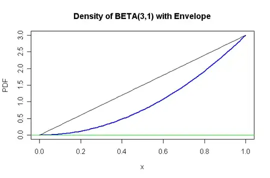
(b) If you wanted to sample from $Beta(3,1)$ using the rejection method, there is a natural nontrivial envelope: you could use the envelope function $3x$ which can be considered a multiple of the triangular density function of $Beta(2,1).$ (It is easy to simulate observations from $Beta(2,1)$ using the inverse CDF method and the envelope is 'close enough' that only a small proportion of candidate values will be rejected.) enter image description here

BruceET
  • 52,418
  • Thanks a lot, thats a great answer. Do you have any tips on finding good envelope functions? – eager2learn Jan 24 '16 at 12:37
  • @eager2learn: I guess more art than science. Important criteria are tightness of envelope fit to the target PDF, and ease of simulation of the PDF on which the envelope is based. Not much is gained by a higher proportion of acceptances if each candidate value is difficult/ slow to generate. Sometimes, the envelope is defined it piece-wise. Also see: `http://math.stackexchange.com/questions/1358708/'. – BruceET Jan 24 '16 at 22:37