3

Smooth classic entropies generalize the standard notions of entropy. This smoothing stands for a minimization/maximization over all events $\Omega$ such that $p(\Omega)\geq 1-\varepsilon$ for a given $\varepsilon\geq 0$. The smooth max and min entropy are defined as:

\begin{equation} H_\infty^\varepsilon (X)= \max_\Omega \min_x(-\log p_{X\Omega}(x)) \end{equation}

\begin{equation} H_0^\varepsilon (X)= \min_\Omega\log \left| x:p_{X\Omega}(x)>0\right| \end{equation}

where $p_{X\Omega}(x)$ is the probability that the event $\Omega$ takes place and $X$ takes the value $x$.

So my question would be, given a specific discrete distribution, for instance something as simple as a fair coin, could someone explicitly compute an example of its smooth max and min entropy?

glS
  • 7,963
Euclean
  • 795
  • I also asked a related question on qc.SE: https://quantumcomputing.stackexchange.com/q/27818/55 – glS Sep 05 '22 at 11:22

2 Answers2

4

I will refer you to this great informal introduction which gives a few finite examples and explains the intuition behind the definitions.

However $H_\infty^\varepsilon$ is not mentioned. The effect of smoothing is similar to $H_0^\varepsilon$, but in reverse: the smoothing will continuously "steal" probability from the most probable states until $\varepsilon$ probability has been stolen. If you have $n$ maximum-probability states and all other states are somewhat less probable, then the maximum probability will be reduced by $\varepsilon/n$. So a single small peak of probability will be smoothed off, but the effect of smoothing will be negligible in two notable cases: if you have many maximum-probability (or close to maximum-probability) states, or if the maximum probability is much greater than $\varepsilon$.

Unlike $H_0^\varepsilon$ which can be radically different from $H_0$, $H_\infty^\varepsilon$ is continuous in $\varepsilon$ in the following sense: $$0<\exp(-H_\infty(X))-\exp(-H_\infty^\varepsilon(X))\le \varepsilon$$ (more generally, $\exp(-H_\infty^\varepsilon(X))$ is an increasing 1-Lipschitz function of $\varepsilon$).

Finally, for a fair coin: $$H_\infty^\varepsilon(X)=-\log \frac{1-\varepsilon}{2}$$ $$H_0^\varepsilon(X)=\begin{cases}\log 2&\varepsilon<1/2\\0&\varepsilon\ge 1/2\end{cases}$$ $H_\infty^\varepsilon$ steals $\varepsilon/2$ from each state since they have both maximal probability. $H_0^\varepsilon$ tries to steal from one minimum-probability state to reduce the number of states: this only succeeds if $\varepsilon\ge 1/2$.

Dominik
  • 20,241
  • Then, for a fair coin $H_0^\epsilon(X)=H_0(X)=1$? – Euclean Jun 07 '12 at 09:08
  • 1
    In fact this is only true for small enough $\varepsilon$ (specifically, $\varepsilon<1/2$): I updated my answer. – Generic Human Jun 08 '12 at 12:40
  • Ok, for $\epsilon>1/2$, that is, once you are allowed to still more than 1/2 your fair coin is $\epsilon$-close to a deterministic distribution with 0 entropy. A little late, but I think I got a good understanding! – Euclean Jul 04 '12 at 10:24
  • the link appears to be broken. Though possibly it sent to these notes, which used to be hosted on the same site, and that happened to be snatched by the web archive: https://web.archive.org/web/20151010115049/http://www.itp.phys.ethz.ch/education/hs12/qit/resources/skript1.pdf. Relevant bit is in page 17 – glS Aug 16 '22 at 22:48
  • 1
    @glS: That presentation seems too formal to match the terse description given in the Answer, but here is an informal write-up with a similar PDF name and on a related URL, "tips02.pdf". – hardmath Sep 05 '22 at 00:12
0

A few examples of calculation of smoothed min-entropy:

(Non-degenerate distribution, small $\epsilon$) Consider a generic discrete probability distribution whose maximum is strictly larger than the other values. We can assume without loss of generality that the probabilities are arranged in non-increasing order, so that we have $$P_{\rm max}\equiv\max_x P_x = P_1 > P_2 \ge P_3 \ge \cdots$$ The min-entropy is in this case $$H_{\rm min}(X)_P\equiv H_{\infty}(X)_P \equiv \log \frac{1}{P_{\rm max}}.$$ On the other hand, for small enough $\epsilon>0$ (or more specifically, for $\epsilon<P_{\rm max}-P_2$), the smoothed min-entropy will be $$H_{\rm min}^\epsilon(X)_P = \log\left( \frac{1}{P_{\rm max}-\epsilon}\right).$$ The idea is simple: we "steal" probability from the maximum probability event, in order to decrease the maximum probability of the distribution. As long as $\epsilon$, the amount we're stealing is small enough, then the most likely event does not change, and we get this result.

(Non-degenerate distribution, not-so-small $\epsilon$) If, on the other hand, $\epsilon$ starts being large enough that the most likely event changes, then we get a different values for the smoothed min-entropy. The next simplest such example we can consider is when $\epsilon$ is large enough to lower $P_{\rm max}$ to the height of $P_2$, but not large enough to also lower $P_{\rm max}$ and $P_2$ to the height of $P_3$. More precisely, this amounts to the conditions: $$\epsilon>P_{\rm max}-P_2, \qquad P_2>P_3, \qquad \epsilon< (P_{\rm max}-P_2) + 2(P_2-P_3).$$ In such cases, we get $$H_{\rm min}^\epsilon(X)_P = \log\left(\frac{1}{P_2 - \left(\frac{\epsilon-(P_{\rm max}-P_2)}{2}\right) }\right) = \log \left(\frac{2}{P_{\rm max}+P_2 - \epsilon}\right).$$ The first expression in the logarithm is derived by gradually removing probability first from $P_{\rm max}$, and then from $P_{\rm max}$ and $P_2$ together: $\epsilon-(P_{\rm max}-P_2)$ is how much probability we have to remove after having $P_{\rm max}=P_2$, and we then decrease both $P_{\rm max}$ and $P_2$ together, but at a halved rate (because we have to decrease them both together, so the "cost" is doubled).

(Degenerate most likely events) Suppose now that $P_1=P_2=\cdots P_n> P_{n+1}\ge ...$ In this scenario, for $\epsilon$ small enough, we reduce all of the most likely events at the same time. Therefore the smoothed min-entropy becomes $$H_{\rm min}^\epsilon(X)_P = \log\left(\frac{1}{P_{\rm max} - \epsilon/n}\right).$$

(More explicit examples)

  • Consider $P_1 = 0.7, P_2=0.2, P_3=0.1$. Then $$H_{\rm min}^\epsilon(X)_P = \begin{cases}\log\left(\frac{1}{0.7-\epsilon}\right) & \epsilon \le 0.5, \\ \log\left(\frac{1}{0.2 - (\epsilon-0.5)/2}\right), & 0.5\le \epsilon\le 0.7, \\ \log\left(\frac{1}{0.1 - (\epsilon-0.7)/3}\right), & 0.7\le \epsilon\le 1 \end{cases}.$$
  • Another example, where this time the two least likely even have the same probability, is $P_1 = 0.8, P_2=0.1, P_3=0.1$. In this case, we have $$H_{\rm min}^\epsilon(X)_P = \begin{cases}\log\left(\frac{1}{0.8-\epsilon}\right) & \epsilon \le 0.7, \\ \log\left(\frac{1}{0.1 - (\epsilon-0.7)/3}\right), & 0.7\le \epsilon\le 1 \end{cases}.$$

Note how $H_{\rm min}^\epsilon(X)_P$ is always continuous, but not smooth, with respect to $\epsilon$. More specifically, here is what the two smoother min-entropies look like as a function of $\epsilon$:

enter image description here

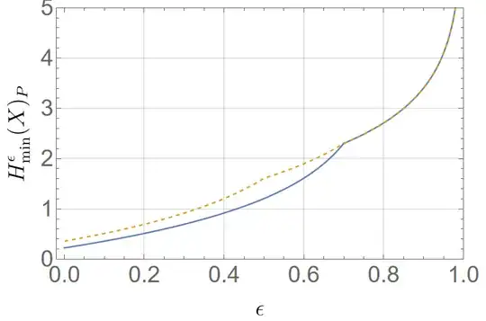
Here, the dashed orange line corresponds to the first example, while the solid blue line to the second one.

glS
  • 7,963