Generating in the computer a bi-dimensional vector which components obey a gaussian distribution from a standard random number generator

Question

I'm showing you an exercise I have tried and I'm looking for your opinion/critic because this is my first time in kinetic theory and stochastic processes and I wish to know if I'm making right, in other words, can you check it and tell me if everything is fine with my answer?

Greetings!

Consider two stochastic variables $X,\,Y\,$ defined both in the interval $\,[-\infty,+\infty],\,$ and suppose they obey a bi-dimensional gaussian distribution, i.e., $$P_{2}(x,y)=\frac{1}{2\pi\sigma^{2}}e^{-(x^{2}+y^{2})/(2\,\sigma^{2})}$$ Now, let's define $\,s=x^{2}+y^{2}\,$ and $\,\phi\,$ the angle formed by the vector of components $(x,y)$ with respect to the positive semi-axis $\,OX\,$ (i.e., the usual polar angle).

Discuss how can be generated in the computer a bi-dimensional vector which components obey a gaussian distribution from a standard random number generator, that gives numbers uniformly distributed between 0 and 1.

What I have done:

Given a standard random number generator. Let $n_{1}, n_{2}$ be the results of two outputs of this number generator. Define $s$ so that: $$\int_{0}^{s} \frac{e^{-z/2\sigma^{2}}}{2\sigma^{2}}dz=1-e^{-s/2\sigma^{2}}=n_{1}$$ So: $s=2\sigma^{2} ln(|1-n_{1}|).$

$\theta=2\pi n_{2}.$

Let $$x=\sqrt{s}\cos(\theta)$$ $$y=\sqrt{s}\sin(\theta).$$ The points $(x,y)$ so generated have the prescribed distribution.

Answer 1

This looks a lot like the Box-Muller method of generating two independent standard normal random variables $Z_1$ and $Z_2$ from two independent standard uniform random variables $U_1$ and $U_2.$ Please check online sources including Wikipedia, Wolfram, any of several on this site, or lecture notes from NYU and CalTech--depending on your mathematical level and whether you are mainly interested in mathematical proofs or computer implementations.

Intuitively, the process may be clearest when considered in reverse. Suppose we have a rifle clamped in a vise and aimed at the bull's eye of a target. Horizontal errors and vertical errors $Z_1$ and $Z_2$, respectively are independently $Norm(0,1).$

Upon converting to polar coordinates, it seems clear that, associated with the position of a random rifle hit, will be an angle $\Theta$ clockwise from the positive half line that is distributed $Unif(0, 2\pi)$. It can be divided by $2\pi$ to give a standard uniform random variable $Unif(0,1).$

The squared distance from the origin to such a random hit point is $$Z_1^2 + Z_2^2 \sim Chisq(2) = Exp(rate = 1/2),$$ which can be divided by $2$ to get a random variable $Q \sim Exp(rate = 1)$ with CDF $P(Q \le t) = F(t) = 1 - e^{-t},$ for $t > 0.$ Then it is easy to show that $e^{-Q} \sim Unif(0,1).$

So starting with two independent standard normal random variables, we have found two standard uniform random variables (which turn out to be independent). The Box-Muller transformation is the inverse of process.

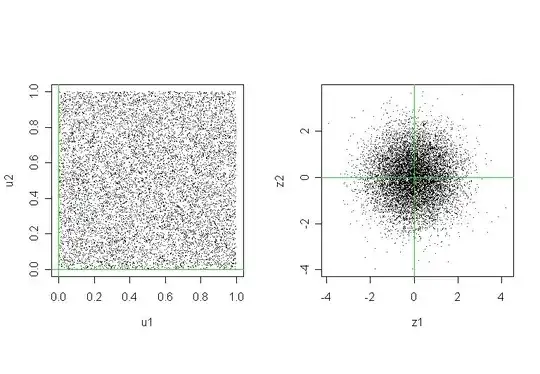
Below is an illustration of the Box-Muller transform starting with 10,000 pairs of uniformly distributed points.

 m = 10000;  u1 = runif(m);  u2 = runif(m)
 z1 = sqrt(-2*log(u1))*cos(2*pi*u2)
 z2 = sqrt(-2*log(u1))*sin(2*pi*u2)
 mean(u1);  var(u1)
 ## 0.5006089    # approx 1/2
 ## 0.08388625   # approx 1/12
 mean(z1);  var(z1)
 ## -0.003667858 # approx 0
 ## 1.016240     # approx 1
 shapiro.test(z1[1:5000])  # Shapiro-Wilk test of normality

 ##   Shapiro-Wilk normality test

 ## data:  z1[1:5000]   # First 50000 (size limit for procedure)
 ## W = 0.9997, p-value = 0.6502  # consistent with normal

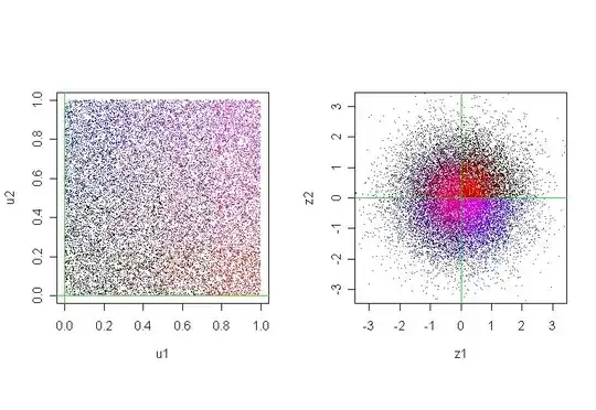
A second simulation uses 16 colors to illustrate the nature of the transformation. A point on the left-hand plot has the same color as its image under the Box-Muller transformation on the right. (A very small percentage of points lie outside the plotting region of the right-hand plot.)