Overfitting in Linear Regression

Question

I'm just getting started with machine learning and I have trouble understanding how overfitting can happen in a linear regression model.

Considering we use only 2 feature variables to train a model, how can a flat plane possibly be overfitted to a set of data points?

I assume linear regression uses only a line to describe the linear relationship between 2 variables and a flat plane to describe the relationship between 3 variables, I have trouble understanding (or rather imagining) how overfitting in a line or a plane can happen?

Answer 1

In linear regression overfitting occurs when the model is "too complex". This usually happens when there are a large number of parameters compared to the number of observations. Such a model will not generalise well to new data. That is, it will perform well on training data, but poorly on test data.

A simple simulation can show this. Here I use R:

> set.seed(2)
> N <- 4
> X <- 1:N
> Y <- X + rnorm(N, 0, 1)
> 
> (m0 <- lm(Y ~ X)) %>% summary()
Coefficients:
            Estimate Std. Error t value Pr(>|t|)
(Intercept)  -0.2393     1.8568  -0.129    0.909
X             1.0703     0.6780   1.579    0.255
Residual standard error: 1.516 on 2 degrees of freedom
Multiple R-squared:  0.5548,    Adjusted R-squared:  0.3321 
F-statistic: 2.492 on 1 and 2 DF,  p-value: 0.2552

Note that we obtain a good estimate of the true value for the coefficient of X. Note the Adjusted R-squared of 0.3321 which is an indication of the model fit.

Now we fit a quadratic model:

> (m1 <- lm(Y ~ X + I(X^2) )) %>% summary()
Coefficients:
            Estimate Std. Error t value Pr(>|t|)
(Intercept)  -4.9893     2.7654  -1.804    0.322
X             5.8202     2.5228   2.307    0.260
I(X^2)       -0.9500     0.4967  -1.913    0.307
Residual standard error: 0.9934 on 1 degrees of freedom
Multiple R-squared:  0.9044,    Adjusted R-squared:  0.7133 
F-statistic: 4.731 on 2 and 1 DF,  p-value: 0.3092

Now we have a much higher Adjusted R-squared: 0.7133 which may lead us to think that the model is much better. Indeed if we plot the data and the predicted valus from both models we get :

> fun.linear <- function(x) { coef(m0)[1] + coef(m0)[2] * x  }
> fun.quadratic <- function(x) { coef(m1)[1] + coef(m1)[2] * x  + coef(m1)[3] * x^2}
> 
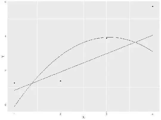
> ggplot(data.frame(X,Y), aes(y = Y, x = X)) + geom_point()  + stat_function(fun = fun.linear) + stat_function(fun = fun.quadratic)

So on the face of it, the quadratic model looks much better.

Now, if we simulate new data, but use the same model to plot the predictions, we get

> set.seed(6)
> N <- 4
> X <- 1:N
> Y <- X + rnorm(N, 0, 1)
> ggplot(data.frame(X,Y), aes(y = Y, x = X)) + geom_point()  + stat_function(fun = fun.linear) + stat_function(fun = fun.quadratic)

Clearly the quadratic model is not doing well, whereas the linear model is still reasonable. However, if we simulate more data with an extended range, using the original seed, so that the initial data points are the same as in the first simulation we find:

> set.seed(2)
> N <- 10
> X <- 1:N
> Y <- X + rnorm(N, 0, 1)
> ggplot(data.frame(X,Y), aes(y = Y, x = X)) + geom_point()  + stat_function(fun = fun.linear) + stat_function(fun = fun.quadratic)

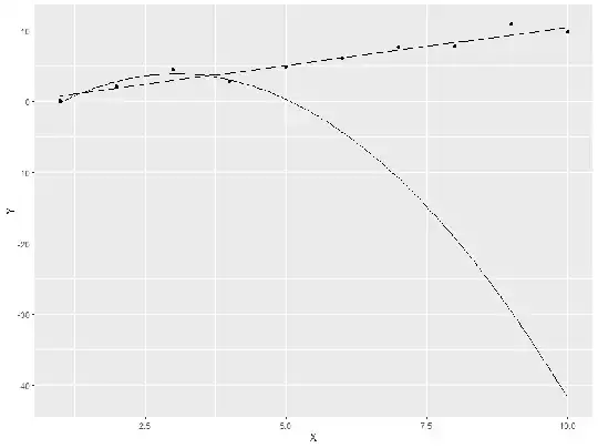
Clearly the linear model still performs well, but the quadratic model is hopeless outside the orriginal range. This is because when we fitted the models, we had too many parameters (3) compared to the number of observations (4).

---

Edit: To address the query in the comments to this answer, about a model that does not include higher order terms.

The situation is the same: If the number of parameters approaches the number of observations, the model will be overfitted. With no higher order terms, this will occur when the number of variables / features in the model approaches the number of observations.

Again we can demonstrate this easily with a simulation:

Here we simulate random data data from a normal distribution, such that we have 7 observations and 5 variables / features:

> set.seed(1)
> n.var <- 5
> n.obs <- 7
> 
> dt <- as.data.frame(matrix(rnorm(n.var * n.obs), ncol = n.var))
> dt$Y <- rnorm(nrow(dt))
> 
> lm(Y ~ . , dt) %>% summary()
Coefficients:
            Estimate Std. Error t value Pr(>|t|)
(Intercept)  -0.6607     0.2337  -2.827    0.216
V1            0.6999     0.1562   4.481    0.140
V2           -0.4751     0.3068  -1.549    0.365
V3            1.2683     0.3423   3.705    0.168
V4            0.3070     0.2823   1.087    0.473
V5            1.2154     0.3687   3.297    0.187
Residual standard error: 0.2227 on 1 degrees of freedom
Multiple R-squared:  0.9771,    Adjusted R-squared:  0.8627 

We obtain an adjusted R-squared of 0.86 which indicates excellent model fit. On purely random data. The model is severely overfitted. By comparison if we double the number of obervations to 14:

> set.seed(1)
> n.var <- 5
> n.obs <- 14
> dt <- as.data.frame(matrix(rnorm(n.var * n.obs), ncol = n.var))
> dt$Y <- rnorm(nrow(dt))
> lm(Y ~ . , dt) %>% summary()
Coefficients:
            Estimate Std. Error t value Pr(>|t|)

(Intercept) -0.10391    0.23512  -0.442   0.6702

V1          -0.62357    0.32421  -1.923   0.0906 .
V2           0.39835    0.27693   1.438   0.1883

V3          -0.02789    0.31347  -0.089   0.9313

V4          -0.30869    0.30628  -1.008   0.3430

V5          -0.38959    0.20767  -1.876   0.0975 .

Signif. codes:  0 ‘*’ 0.001 ‘’ 0.01 ‘*’ 0.05 ‘.’ 0.1 ‘ ’ 1
Residual standard error: 0.7376 on 8 degrees of freedom
Multiple R-squared:  0.4074,    Adjusted R-squared:  0.03707 
F-statistic:   1.1 on 5 and 8 DF,  p-value: 0.4296

..adjusted R squared drops to just 0.037

Answer 2

Large number of parameters compared to data points

In general, one aspect of overfitting is trying to "invent information out of nothing" when you want to determine a comparably large number of parameters from a limited amount of actual evidence data points.

For a simple linear regression y = ax + b there are two parameters, so for most sets of data it would be underparametrised, not overparametrised. However, let's look at the (degenerate) case of only two data points. In that situation you can always find a perfect linear regression solution - however, is that solution necessarily meaningful? Possibly not. If you treat the linear regression of two data points as a sufficient solution, that would be a prime example of overfitting.

Here is a nice example of overfitting with a linear regression by Randall Munroe of xkcd fame that illustrates this issue:

Answer 3

Overfitting happens when the model performs well on the train data but doesn't do well on the test data. This is because the best fit line by your linear regression model is not a generalized one. This might be due to various factors. Some of the common factors are

• Outliers in the train data.
• Train and Test data are from different distributions.

So before building the model ensure that you have checked up on these factors to get a generalized model.