I followed from this question1,question2.
I have the following task to do: I have time series data. Training by the consecutive 3 days to predict the each 4th day. Each day data represents one CSV file which has dimension 24x25. Every data points of each CSV file are pixels.
Now I need to do that, predict day4 (meaning the 4th day) by using training data day1, day2, day3 (meaning the three consecutive days prior), and after that calculate MSE between predicted day4 data and original day4 data. Let's call it mse1.
Similarly, I need to predict the day5 (meaning the 5th day) by using training data day2, day3, day4, and then calculate the mse2 (MSE between predicted day5 data and original day5 data).
I need to predict day6 (meaning the 6th day) by using training data day3, day4, day5, and then calculate mse3 (MSE between predicted day6 data and original day6).
..........
And finally I want to predict day93 by using training data day90, day91, day92, calculate mse90 (MSE between predicted day93 data and original day93).
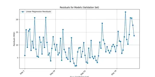
I want to use in this case, Linear regression, and we have 90 MSE for this model.
import os
import pandas as pd
import numpy as np
from sklearn.linear_model import LinearRegression, Ridge
from sklearn.preprocessing import MinMaxScaler
import matplotlib.pyplot as plt
from tensorflow.keras.models import Sequential
from tensorflow.keras.layers import LSTM, Dense
Paths
data_folder = r'C:\Users\alokj\OneDrive\Desktop\jupyter_proj\All_data'
output_folder = r'C:\Users\alokj\OneDrive\Desktop\jupyter_proj\90_days_merged'
Ensure the output folder exists
os.makedirs(output_folder, exist_ok=True)
List all CSV files in the folder
csv_files = [f for f in os.listdir(data_folder) if f.endswith('.csv')]
Sort the files based on the numeric part extracted from the filename
csv_files = sorted(csv_files, key=lambda x: int(x.split('Day')[1].split('')[0]))
Prepare data
data_list = [pd.read_csv(os.path.join(data_folder, file), header=None).values for file in csv_files]
data_array = np.array(data_list)  # Shape: (num_days, 24, 25)
Flatten the data for easier handling in regression models
num_days, rows, cols = data_array.shape
data_flattened = data_array.reshape(num_days, -1)  # Shape: (num_days, 600)
Prepare features and target matrix for range (3, num_days)
X = np.array([data_flattened[i-3:i].flatten() for i in range(3, num_days)])  # Shape: (num_days-3, 1800)
y = data_flattened[3:num_days]  # Target is the 4th day in each sequence
Train-Test Split and Validation (Separate fixed split)
print(len(data_flattened)) #1877
train_size = int(0.8 * len(data_flattened)) # 80% for training
#print(data_flattened[train_size])
print(train_size)  #1501
test_size = len(data_flattened)-train_size
print(test_size)  #376
X_train = X[:train_size]
y_train = y[:train_size]
X_test = X[train_size:]
y_test = y[train_size:]
Scaling the data
scaler_X = MinMaxScaler()
scaler_X.fit(X_train)  # Fit on training set
X_train_scaled = scaler_X.transform(X_train)
X_test_scaled = scaler_X.transform(X_test)
scaler_y = MinMaxScaler()
scaler_y.fit(y_train)  # Fit on training set
y_train_scaled = scaler_y.transform(y_train)
y_test_scaled = scaler_y.transform(y_test)
Scaled version of all data for naive prediction
data_flattened_scaled = scaler_X.transform(data_flattened)
Linear Regression
lr_model = LinearRegression()
lr_model.fit(X_train_scaled, y_train_scaled)
#y_pred_test_scaled_lr = lr_model.predict(X_test_scaled)
#y_pred_test_lr = scaler_y.inverse_transform(y_pred_test_scaled_lr)
#print(data_flattened)
Validation for Days 3 to 93
XX = X_test_scaled[:90]
yy = y_test[:90]
yy_pred_lr = lr_model.predict(XX)
yy_pred_lr = scaler_y.inverse_transform(yy_pred_lr)
Calculate residuals for Linear Regression
residuals_lr = [np.mean((yy[i] - yy_pred_lr[i])**2) for i in range(len(yy))]
Plot residuals for all models
days = [f'Day {i+1}' for i in range(len(residuals_lr))]  # Start labels from Day 4 to Day 93
plt.figure(figsize=(12, 6))
plt.plot(days, residuals_lr, label='Linear Regression Residuals', marker='o')
Configure plot
plt.xticks(ticks=range(0, len(days), 25), labels=[f'Day {i+1}' for i in range(0, len(days), 25)], rotation=45, ha='right')
plt.xlabel('Days (Validation Set)')
plt.ylabel('Residuals (MSE)')
plt.title('Residuals for Models (Validation Set)')
plt.legend()
plt.grid(True)
Save and show plot
plt.savefig(os.path.join(output_folder, 'residuals_plot_models_comparison_with_naive.png'))
plt.show()
We know that linear regression models often do not do very well with time series data because the assumption of independent and identically distributed data is usually violated.
Actually I have implemented my code based on suggestions of @RobertLong's answer1,answer2 from my above linked questions.
Although I am getting expected result, would anybody check my regression model inside the code (if I made any mistakes or bugs that I might not be aware of)?
My all 93 days data folder link that I used for code.
