Time series predictions with LSTM

Question

I have collection of TEC data.My data sample for example the day1,day2,day3,day4.

Case1:

I have the following task to do: Training by the consecutive 3 days to predict the each 4th day. Each day data represents one CSV file which has dimension 24x25. Every datapoints of each CSV file are pixels.

Now, I need to do that, predict day4(means 4th day) by using training data day1, day2, day3(means three consecutive days), after then calculate mse between predicted day4 data and original day4 data. Let's call it mse1.

Similarly, I need to predict the day5 (means 5th day) by using training data day2, day3, day4, and then calculate the mse2(mse between predicted day5 data and original day5 data)

I need to predict day6(means 6th day)by using training data day3, day4, day5, and then calculate mse3(mse between predicted day6 data and original day6)

..........

And finally I want to Predict day93 by using training data day90, day91, day92,calculate mse90(mse between predicted day93 data and original day93)

I want to use in this case LSTM model. And we have 90 mse for lstm model.

Case2:

Here I am using, is known as "the" naive forecast, or a "random walk" forecast.

Naive approach is:

The guess for any day is simply the map of the previous day. I mean simply guess that day2 is the same as day1, guess that day3 is same as day2, guess that day4 is same as day3,....., guess that day91 is same as day90. I mean Predict next day's data using current day's data(predicted_data = current_day_data). Then calculate mse between next_day_data and current_day_data.

import os
import pandas as pd
import numpy as np
from sklearn.linear_model import LinearRegression, Ridge
from sklearn.preprocessing import MinMaxScaler
import matplotlib.pyplot as plt
from tensorflow.keras.models import Sequential
from tensorflow.keras.layers import LSTM, Dense
Paths
data_folder = r'C:\Users\alokj\OneDrive\Desktop\jupyter_proj\All_New_serialdata99_16'
output_folder = r'C:\Users\alokj\OneDrive\Desktop\jupyter_proj\90_days_merged'
Ensure the output folder exists
os.makedirs(output_folder, exist_ok=True)
List all CSV files in the folder
csv_files = [f for f in os.listdir(data_folder) if f.endswith('.csv')]
Sort the files based on the numeric part extracted from the filename
csv_files = sorted(csv_files, key=lambda x: int(x.split('Day')[1].split('')[0]))
Prepare data
data_list = [pd.read_csv(os.path.join(data_folder, file), header=None).values for file in csv_files]
data_array = np.array(data_list)  # Shape: (num_days, 24, 25)
Flatten the data for easier handling in regression models
num_days, rows, cols = data_array.shape
data_flattened = data_array.reshape(num_days, -1)  # Shape: (num_days, 600)
Prepare features and target matrix for range (3, num_days)
X = np.array([data_flattened[i-3:i].flatten() for i in range(3, num_days)])  # Shape: (num_days-3, 1800)
y = data_flattened[3:num_days]  # Target is the 4th day in each sequence
Train-Test Split and Validation (Separate fixed split)
train_size = int(0.8 * len(X))  # 80% for training
print(train_size)
X_train = X[:train_size]
y_train = y[:train_size]
X_test = X[train_size:]
y_test = y[train_size:]
Scaling the data
scaler_X = MinMaxScaler()
scaler_X.fit(X_train)  # Fit on training set
X_train_scaled = scaler_X.transform(X_train)
X_test_scaled = scaler_X.transform(X_test)
scaler_y = MinMaxScaler()
scaler_y.fit(y_train)  # Fit on training set
y_train_scaled = scaler_y.transform(y_train)
y_test_scaled = scaler_y.transform(y_test)
XX = X_test_scaled[:90]
yy = y_test[:90]  # Target for validation
LSTM Model
Reshape data for LSTM (num_samples, timesteps, features)
X_train_lstm = X_train_scaled.reshape(X_train_scaled.shape[0], 3, -1)
#y_train_lstm = y_train_scaled.reshape(y_train_scaled.shape[0], 3, -1)
X_test_lstm = X_test_scaled.reshape(X_test_scaled.shape[0], 3, -1)
XX_lstm = XX.reshape(XX.shape[0], 3, -1)
LSTM Model
lstm_model = Sequential([
    LSTM(64, activation='tanh', return_sequences=False, input_shape=(3, X_train_lstm.shape[2])),
    Dense(y_train_scaled.shape[1])
])
lstm_model.compile(optimizer='adam', loss='mse')
lstm_model.fit(X_train_lstm, y_train_scaled, epochs=20, batch_size=16, verbose=1)
Validation using LSTM
yy_pred_lstm = lstm_model.predict(XX_lstm)
yy_pred_lstm = scaler_y.inverse_transform(yy_pred_lstm)
Calculate residuals for LSTM
residuals_lstm = [np.mean((yy[i] - yy_pred_lstm[i])**2) for i in range(len(yy))]
Naive Prediction
residuals_naive = [np.mean((X_test[i] - X_test[i - 1]) ** 2) for i in range(1, 91)]
Plot residuals for all models
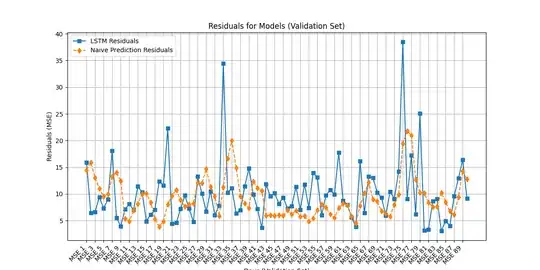
days = [f'Day {i+1}' for i in range(90)]  # Start labels from Day 4 to Day 93
plt.figure(figsize=(12, 6))
plt.plot(days, residuals_lstm, label='LSTM Residuals', marker='s')
plt.plot(days, residuals_naive, label='Naive Prediction Residuals', marker='d', linestyle='--')
Configure plot
plt.xticks(ticks=range(0, len(days), 2), labels=[f'MSE {i+1}' for i in range(0, len(days), 2)], rotation=45, ha='right')
plt.xlabel('Days (Validation Set)')
plt.ylabel('Residuals (MSE)')
plt.title('Residuals for Models (Validation Set)')
plt.legend()
plt.grid(True)
Save and show plot
plt.savefig(os.path.join(output_folder, 'models_comparison_with_naive.png'))
plt.show()

My output result:

I have read many research paper, and they are saying LSTM will be working well on TEC data, although not mentioned anything regarding naive method. And my output graph showing both LSTM and naive both are competitive. My question is, anybody review my specially lstm model code, any flaw inside the code that I am not aware of?

Answer 1

Looking at your TEC data predictions, I think you've built a solid LSTM implementation, but I see why you might be confused about the naive model performing so competitively. Let me share some thoughts that might help:

First off, I noticed you're flattening those 24x25 pixel maps into a 1D array. While this works, you're potentially losing the spatial relationships in your data. Since TEC maps have spatial patterns, have you thought about using a ConvLSTM instead? That way you'd preserve both the temporal and spatial features.

Your LSTM architecture looks reasonable with 64 units and the right input shape for your 3-day window. I might play around with different unit counts (32 or 128) to see if that helps the model outperform the naive forecast more consistently.

For your training approach, 20 epochs is a good start, but I'd suggest adding early stopping to prevent overfitting:

from tensorflow.keras.callbacks import EarlyStopping
early_stopping = EarlyStopping(monitor='val_loss', patience=5, restore_best_weights=True)
lstm_model.fit(X_train_lstm, y_train_scaled, epochs=50, batch_size=16, 
               validation_split=0.2, callbacks=[early_stopping])

I don't see a validation split in your training - that would help you monitor how well the model generalizes during training.

About the naive forecast performing surprisingly well - this happens often with time series data! It could mean:

• You might need more training data for the LSTM to learn meaningful patterns
• The day-to-day TEC patterns might not have enough temporal complexity for LSTM to show its strengths
• The spatial information needs better representation

One quick thing I'd try is tuning your hyperparameters with something like Keras Tuner:

import keras_tuner as kt
def build_model(hp):
    model = Sequential()
    model.add(LSTM(
        hp.Int('units', min_value=32, max_value=128, step=32),
        activation='tanh', 
        return_sequences=False, 
        input_shape=(3, X_train_lstm.shape[2])
    ))
    model.add(Dense(y_train_scaled.shape[1]))
    model.compile(optimizer='adam', loss='mse')
    return model
tuner = kt.RandomSearch(
    build_model, objective='val_loss', max_trials=5, executions_per_trial=3)
tuner.search(X_train_lstm, y_train_scaled, epochs=20, validation_split=0.2)

Also, are there any additional features you could include - like seasonal patterns or time of day effects?

Your evaluation and visualization look good. Consider adding error bars to your plot to show the variability in those MSE values.

Don't be discouraged by the naive model's performance - it's actually a strong baseline for many forecasting problems! It's giving you valuable information about the nature of your data.

Answer 2

As @s-m request here the review

I took a good look at your TEC forecasting code, and I can see why you're puzzled about the LSTM not outperforming the naive approach more clearly. Let me share some thoughts in a more accessible way.

Your code has a solid foundation! The way you've set up the data pipeline, created your prediction system, and compared the methods shows you know what you're doing. But there are a few tweaks that might help your LSTM shine brighter.

First, those 24x25 pixel maps - when you flatten them into one long array, you're basically telling your model "forget these are 2D images." That's like taking a photo of clouds and stretching it into a line! LSTMs are great with sequences but not so much with spatial patterns. Since TEC maps are very much spatial, maybe try a ConvLSTM that can handle both the "where" and "when" aspects of your data.

About Keras Tuner - think of it as your personal assistant that tries different combinations of settings (like knobs on a mixing board) to find what works best. Here's how you might use it:

import keras_tuner as kt
This function tells Keras Tuner what to adjust
def build_model_to_tune(hp):
    model = Sequential()
# Let Keras Tuner decide how many neurons to use (between 32-256)
lstm_units = hp.Int('lstm_units', 32, 256, step=32)

# Let it decide if dropout would help (0-50%)
dropout = hp.Float('dropout', 0, 0.5, step=0.1)

# Build the model with these trial settings
model.add(LSTM(lstm_units, input_shape=(3, X_train_lstm.shape[2])))
model.add(tf.keras.layers.Dropout(dropout))
model.add(Dense(y_train_scaled.shape[1]))

# Let it try different learning rates
lr = hp.Float('learning_rate', 1e-4, 1e-2, sampling='log')
model.compile(optimizer=tf.keras.optimizers.Adam(learning_rate=lr), loss='mse')

return model


Create the tuner and let it search
tuner = kt.BayesianOptimization(
    build_model_to_tune,
    objective='val_loss',
    max_trials=20,  # Try 20 different combinations
    directory='my_tuning_results',
    project_name='tec_lstm_tuning'
)
Run the search with early stopping
tuner.search(
    X_train_lstm, y_train_scaled,
    epochs=50,
    validation_split=0.2,
    callbacks=[tf.keras.callbacks.EarlyStopping(patience=5)]
)
Get the winner
best_model = tuner.get_best_models(1)[0]

Don't worry if the naive model is competitive - that actually tells you something interesting about your data! Sometimes day-to-day patterns in TEC maps might be fairly consistent, which is why "tomorrow looks like today" can be a decent guess.

A few other friendly tips:

• Try adding dropout (like 20-30%) to help your LSTM generalize better
• Definitely add validation during training to watch for overfitting
• Maybe experiment with different sequence lengths (more than 3 days?)
• Consider adding seasonal patterns if TEC has yearly cycles

Would you like me to expand on any part of this?

also here ConvLSTM for Your TEC Forecasting

Let's talk about using ConvLSTM for your TEC data. It's like giving your model "spatial awareness" along with time memory

The ConvLSTM Advantage for TEC Maps

Think about your TEC data as weather maps changing over time. A regular LSTM treats each pixel separately without understanding that nearby pixels are related. ConvLSTM actually "sees" the patterns across the 24x25 grid while also tracking how they evolve

Here's a simple way to start with ConvLSTM:

from tensorflow.keras.layers import ConvLSTM2D, Flatten, Dense
from tensorflow.keras.models import Sequential
Reshape your data to keep the spatial structure
Instead of flattening to 1D arrays!
X_train_convlstm = np.zeros((train_samples, 3, 24, 25, 1))  # 3 days of 24x25 maps
Fill in your data
for i in range(train_samples):
    for day in range(3):
        X_train_convlstm[i, day, :, :, 0] = your_original_data[i+day]
Build a simple ConvLSTM model
model = Sequential([
    ConvLSTM2D(64, kernel_size=(3, 3), padding='same', 
              input_shape=(3, 24, 25, 1), activation='relu'),
    Flatten(),
    Dense(24*25)  # Output reshaped to match your TEC map dimensions
])
model.compile(optimizer='adam', loss='mse')

If you're enjoying working with ConvLSTMs, here are some great resources to dive deeper:

Academic Papers

1. Original ConvLSTM Paper: "Convolutional LSTM Network: A Machine Learning Approach for Precipitation Nowcasting" by Shi et al. - This started it all

2. Weather Forecasting Applications: "Deep Learning for Precipitation Nowcasting: A Benchmark and A New Model" - Very relevant to your TEC forecasting task.

3. Ionospheric TEC Forecasting: "Forecasting the Ionosphere Using Convolutional LSTMs for Space Weather Applications" - Specifically about TEC forecasting

Practical Tutorials & Code

1. Keras Documentation: ConvLSTM2D Layer Guide - Official documentation with parameters explained

2. GitHub Example: Time Series Prediction with ConvLSTM - Shows implementation in PyTorch with visual examples

3. TensorFlow Tutorial: Spatio-temporal forecasting with ConvLSTM - Great tutorial with moving MNIST example

Video Explanations

1. "ConvLSTM Explained" - short course

Remember, the reshape of your data is crucial - that's the main difference from regular LSTM! Your input needs to have shape: (samples, timesteps, height, width, channels).

Answer 3

As @adithya-bandara mentioned, your code flattened the 2D TEC maps and used a basic LSTM, which lost spatial information and correlations. As an alternative approach, I replaced the LSTM with a ConvLSTM2D model that preserves both spatial and temporal patterns by directly using the 24×25 grid. I also reshaped the data to 5D to match ConvLSTM2D’s input requirements, normalized the full dataset consistently, added BatchNormalization and EarlyStopping for better training, and used Conv3D as the output layer to reconstruct the predicted TEC map:

import os
import numpy as np
import pandas as pd
from tensorflow.keras.models import Sequential
from tensorflow.keras.layers import ConvLSTM2D, BatchNormalization, Conv3D
from tensorflow.keras.callbacks import EarlyStopping
from sklearn.preprocessing import MinMaxScaler
import matplotlib.pyplot as plt
Paths
data_folder = r'C:\Users\alokj\OneDrive\Desktop\jupyter_proj\All_New_serialdata99_16'
output_folder = r'C:\Users\alokj\OneDrive\Desktop\jupyter_proj\90_days_merged'
os.makedirs(output_folder, exist_ok=True)
Load and sort data
csv_files = sorted([f for f in os.listdir(data_folder) if f.endswith('.csv')],
                   key=lambda x: int(x.split('Day')[1].split('')[0]))
Load TEC maps: shape (days, height, width)
data = [pd.read_csv(os.path.join(data_folder, f), header=None).values for f in csv_files]
data = np.array(data)  # shape: (93, 24, 25)
Normalize TEC data (MinMax over whole dataset)
scaler = MinMaxScaler()
data_reshaped = data.reshape(len(data), -1)
data_scaled = scaler.fit_transform(data_reshaped).reshape(-1, 24, 25)
Build input-output pairs
X, y = [], []
for i in range(3, len(data_scaled)):
    X.append(data_scaled[i-3:i])  # shape: (3, 24, 25)
    y.append(data_scaled[i])      # shape: (24, 25)
X = np.array(X)[-90:]  # shape: (90, 3, 24, 25)
y = np.array(y)[-90:]  # shape: (90, 24, 25)
Reshape for ConvLSTM2D: (samples, time, rows, cols, channels)
X = X[..., np.newaxis]  # (90, 3, 24, 25, 1)
y = y[..., np.newaxis]  # (90, 24, 25, 1)
Train/val split
train_size = int(0.8 * len(X))
X_train, y_train = X[:train_size], y[:train_size]
X_val, y_val = X[train_size:], y[train_size:]
Build ConvLSTM2D model
model = Sequential([
    ConvLSTM2D(filters=32, kernel_size=(3, 3), activation='tanh',
               input_shape=(3, 24, 25, 1), return_sequences=False),
    BatchNormalization(),
    Conv3D(filters=1, kernel_size=(3, 3, 1), activation='sigmoid', padding='same')
])
model.compile(optimizer='adam', loss='mse')
early_stop = EarlyStopping(monitor='val_loss', patience=5, restore_best_weights=True)
model.fit(X_train, y_train, epochs=50, batch_size=8, validation_data=(X_val, y_val), callbacks=[early_stop], verbose=1)
Predict and calculate MSE per frame
y_pred = model.predict(X_val)
y_pred_inv = scaler.inverse_transform(y_pred.reshape(len(y_pred), -1))
y_true_inv = scaler.inverse_transform(y_val.reshape(len(y_val), -1))
mse_list = [np.mean((y_pred_inv[i] - y_true_inv[i])**2) for i in range(len(y_val))]
Plot MSEs
plt.figure(figsize=(12, 6))
plt.plot(range(1, len(mse_list)+1), mse_list, marker='o')
plt.xlabel('Day Index (Relative to Validation Start)')
plt.ylabel('MSE')
plt.title('ConvLSTM2D MSE per Day (Validation)')
plt.grid(True)
plt.savefig(os.path.join(output_folder, 'conv_lstm_mse_plot.png'))
plt.show()