Background
Another Description
A fairly detailed
image-less description and proof exists in the "Kinoshita's Example"
section (pages 334-376 of the PDF) of the slides for the talk
"Advanced Fixed Point Theory" by Andy McLennan for the January
2017 School on "Equilibria in Games: existence, selection
and dynamics" .
Terminology
While the OP uses Kinoshita's "sponge roll" analogy, according
to the literature (e.g. Bing and McLennan), this example of Kinoshita
has been called a "(tin) can with a roll of toilet paper". For
convenience, I will refer to $A_{1}$ as "the base",
$A_{3}$ as "the side", and $A_{2}$ as "the roll".
Code
I will generate various images with Mathematica, and will
keep some condensed code in an appendix at the end, referenced by number throughout.
While it is not as interactive, the core Wolfram
Engine is free for non-commercial
personal use so that you
could run this code and generate images from the post with something
like Export["C:\\blah.png",(*code here*)].
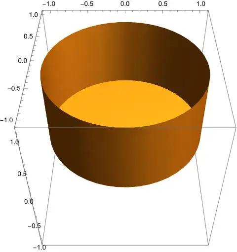
The Set $A$
The base $A_{1}$ is the open unit disk in the plane $z=0$. And the
side $A_{3}$ is a closed cylinder of radius and height $1$. Together,
they can be plotted with $0\le\varphi<2\pi$ with code like 1:
$A_{2}$ is a bit different in that it requires $\varphi$ to range
over all non-negative values. Since $A_{2}$ allows $z$ to vary freely
between $0$ and $1$, it is a prism over the polar curve $r=\dfrac{2}{\pi}\arctan\varphi$,
which we can graph in the $xy$-plane. While a precise graph for all
$\varphi$ is not possible to graph because the roll approaches the
side cylinder, we can see all reasonable detail for $0\le\varphi\le100\pi$
with code like 2:
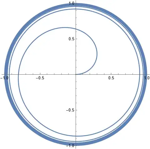
Note that this curve is also the intersection between the base and
the roll $A_{1}\cap A_{2}$. The other pairwise intersections are
empty.
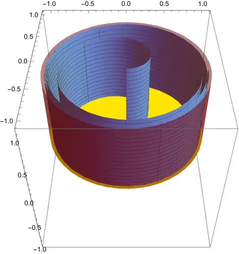
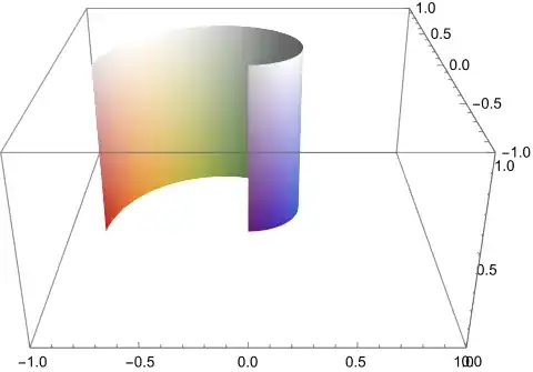
For a 3D picture of the whole of $A$, we might only use $0\le\varphi\le6\pi$
for the roll and produce something like this (3):
Images Under $f$
We will work through these in order of increasing complexity.
Image of the side $A_{3}$
Understanding $f$
The restriction of $f$ to the side is defined relatively simply,
but still involves cases and is worth analyzing. With a little bit
of algebra, we have
$$f(1,\varphi,z)=\begin{cases}
\left(1,\varphi+\pi(2z)-\pi,\frac{3}{4}(2z)\right) & \text{ for }0\le2z\le1\\
\left(1,\varphi+\pi(2z-1),\frac{3}{4}+\frac{1}{4}(2z-1)\right) & \text{ for }0\le2z-1\le1
\end{cases}\text{.}$$
Note that this is well-defined (and continuous) because the angle
components are equal (by the original definition) and when $z=\dfrac{1}{2}$,
the height components of both cases are $\dfrac{3}{4}$.
Also, the radius component is always $1$, so that $f$ maps $A_{3}$
into $A_{3}$.
Case I: Lower Cylinder
For now, let's focus on the first case. As $z$ increases from $0$
to $\dfrac{1}{2}$, the height component of the output increases from
$0$ to $\dfrac{3}{4}$, so that there is a sort of vertical stretch
of the lower half of the side. In addition, the angle shift $\pi(2z)-\pi$
increases from $-\pi$ to $0$ as $z$ increases, so there is a sort
of twisting. For example:
- The top circle at $z=\dfrac{1}{2}$ is raised to $z=\dfrac{3}{4}$
with no twist.
- The middle circle at $z=\dfrac{1}{4}$ is raised to $z=\dfrac{3}{8}$
with a quarter-turn due to $\varphi-\dfrac{\pi}{2}$.
- The bottom circle at $z=0$ is not raised, but is given a half-turn
due to $\varphi-\pi$.
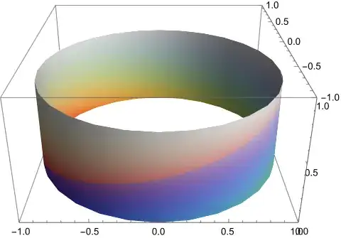
We can visualize this by coloring the lower half of the side based
on $\varphi$ and lightening it as $z$ increases, and then using
the same coloring/shading for the corresponding image points. This
lower half is given by 4:
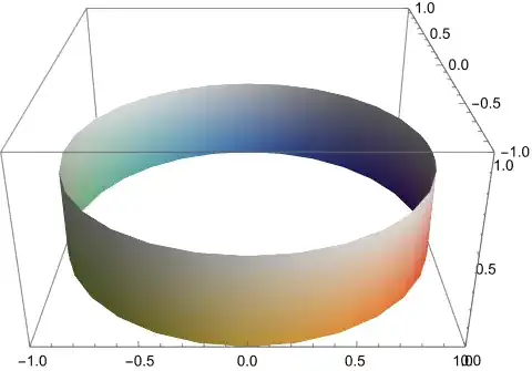
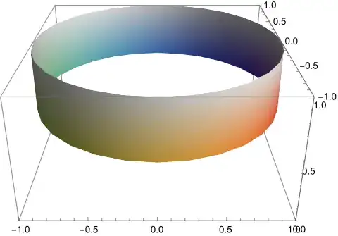
And it is mapped onto the lower third to look like this (5):
Case II: Upper Cylinder
For the second case, things are very similar. As $z$ increases from
$\dfrac{1}{2}$ to $1$, the height component of the output increases
from $\dfrac{3}{4}$ to $1$, so that there is a sort of vertical
compression of the upper half of the side. In addition, the angle
shift $\pi(2z-1)$ increases from $0$ to $\pi$ as $z$ increases,
so there is again a sort of twisting. For example:
- The bottom circle at $z=\dfrac{1}{2}$ is raised to $z=\dfrac{3}{4}$
with no twist.
- The middle circle at $z=\dfrac{3}{4}$ is raised to $z=\dfrac{7}{8}$
with a quarter-turn (in the opposite direction of case I) due to $\varphi+\dfrac{\pi}{2}$.
- The top circle at $z=1$ is not raised, but is given a half-turn due
to $\varphi+\pi$.
We can visualize this with coloring in a similar manner as for case
I. by coloring the lower half of the side based on $\varphi$ and
lightening it as $z$ increases, and then using the same coloring/shading
for the corresponding image points. This lower half is given by 6:
And it is mapped onto the lower third to look like this (note that
the twisting is faster than case I to compensate for the compressed
height range) (see 7):

Entire Side
Because $f$ sends the side to itself in two relatively-simple cases,
it's very reasonable to show this restriction of $f$ all at once.
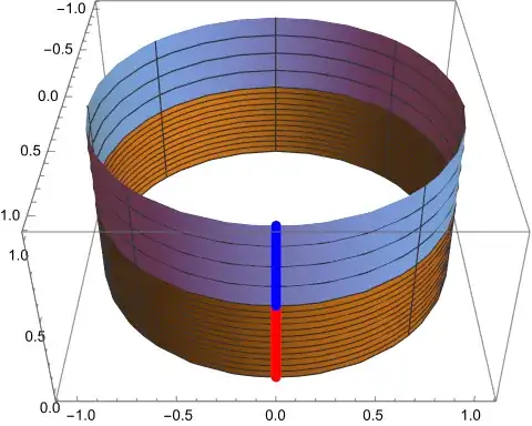
In order to see the twist and height deformations more precisely,
we can highlight $\varphi=0,\dfrac{\pi}{4},\ldots,\dfrac{7\pi}{4}$
(with special focus on $\varphi=0$) and values of $z$ that will
end up equally-spaced.
The entire domain might then look something like this (8):
This choice of viewpoint and curves lets us learn a lot by looking
at the corresponding image (9):
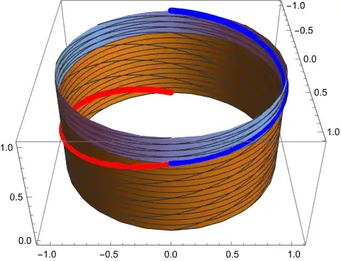
Note the kink in the curves of constant (input) $\varphi$ due to
the change in cases.
Image of the base $A_{1}$
Understanding $f$
The restriction of $f$ to the base is defined a little unusually
in terms of cases with $\vartheta$, so let's unpack that before trying
to understand what $f$ does. Specifically, we have different cases
for $\vartheta(r)\ge\pi$ and $\vartheta(r)\le\pi$. Note that $\vartheta(r)=\tan\dfrac{\pi r}{2}$
is increasing for $0\le r<1$, so we can write the cases in terms
of $r$. $\vartheta(r_{0})=\pi$ is satisfied when $\tan\dfrac{\pi r_{0}}{2}=\pi$,
so that $r_{0}=\dfrac{2}{\pi}\arctan\pi\approx0.8$ (10). Therefore, we may write
the restriction of $f$ to $A_{1}$ as
$$f(r,\varphi,0)=\begin{cases}
\left(\frac{2}{\pi}\arctan\left(\tan\frac{\pi r}{2}-\pi\right),\varphi-\pi,0\right) & \text{ for }r\ge r_{0}\\
\left(0,0,1-\frac{1}{\pi}\tan\frac{\pi r}{2}\right) & \text{ for }r\le r_{0}
\end{cases}$$
Note that this is well-defined (and continuous) because when $r=r_{0}$
so that $\tan\dfrac{\pi r}{2}=\pi$, the radius component of the first
case reduces to $0$ (so that the point is the origin and the angle
component is irrelevant), and the height component of the second case
also reduces to $0$.
Case I: Outer Ring to Disk
For now, let's focus on the first case. It's clear from trigonometry
that the radius component is an increasing function. In fact, a plot
(starting from $r=r_{0}$) looks like this: 11

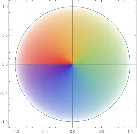
What this means is that the outer annulus for $r_{0}\le r<1$ is stretched
to fill the entire disk $A_{1}$, and also rotated by an angle of
$\pi$ (because of the $\varphi-\pi$ in the angle component).
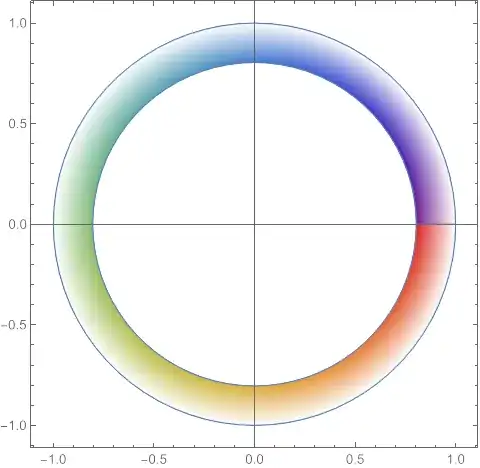
We can visualize this by coloring that part of the domain based on
$\varphi$ and lightening it as $r$ increases, and then using the
same coloring/shading for the corresponding image points. This part
of the domain is given by 12:
And it is mapped onto the whole disk to look like this: 13
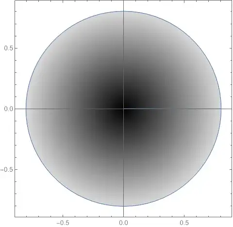
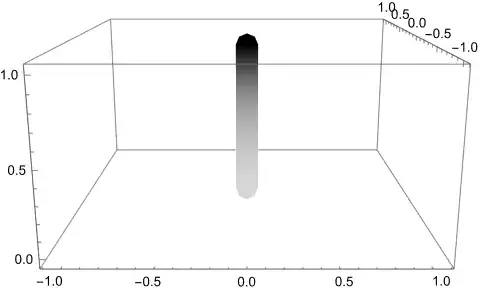
Case II: Inner Disk to Segment
For the second case, note that $1-\dfrac{\vartheta(r)}{\pi}$ decreases
from $1$ to $0$ as $r$ increases from $0$ to $r_{0}$. 14
produces 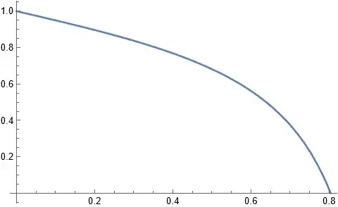
Since the radius component of $f$ is $0$ in this case, the entire
inner disk of radius $r_{0}$ is mapped to a vertical line segment
(part of the roll $A_{2}$), with the center of the disk mapped to
the highest point, and the rest stretched from there based on radius.
Since the angle $\varphi$ doesn't affect the output, there is no
reason to color based on angle. This part of the domain is given by
15
And it is mapped onto the (exaggerated) vertical line segment like
this: 16
(Since the second case is so different, there is probably little benefit
in trying to show both cases in a single image.)
Image of the roll $A_{2}$
This portion is saved for last not just because it is more complicated,
but because the sorts of patterns we've seen in the other two parts
will come up again here.
Unrolling for $f$
Since the roll $A_{2}$ is coiled up via $r=\dfrac{2}{\pi}\arctan\varphi$,
it could be hard to understand partitions of it (or notatble curves
in it) from a 3D picture. Therefore, we can instead view points in
the "unrolled" $\varphi z$-plane (specifically, the infinite
half-strip of height $1$) as corresponding to the relevant points
in $A_{2}$.
And since all three cases of $f$ have the form $\left(\dfrac{2}{\pi}\arctan\theta,\theta,\zeta\right)$,
the image of $A_{2}$ under $f$ lies within $A_{2}$, so that we
can always view the image in the $\theta\zeta$-plane (withe the same
correspondence to points in $A_{2}$ as the input $\varphi z$-plane),
safely ignoring the radius component.
Case I Components: $g$ and $h$
The rectangle in the input $\varphi z$-plane corresponding to $0\le\varphi\le\pi$,
$0\le z\le1$ is mapped by $f$ to some region of the output plane
via
$$(\varphi,z)\mapsto\left(\varphi+\pi g\left(\frac{\varphi}{\pi},z\right),z+h\left(\frac{\varphi}{\pi},z\right)\right)$$
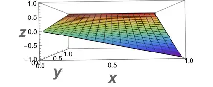
In order to understand what this does, we will need to understand
$g$ and $h$. $g(x,y)=(-x)(1-y)+y$ (defined in 17), so that as $y$ increases from $0$ to $1$,
$g$ interpolates linearly from $-x$ to $1$. We can graph $z=g(x,y)$
with code like 18 to produce:
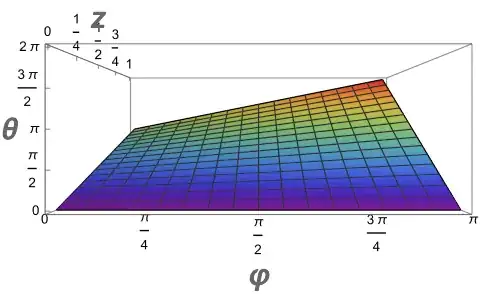
In our particular context, as $z$ increases from $0$ to $1$, the
angle $\theta=\varphi+\pi g\left(\dfrac{\varphi}{\pi},z\right)$ interpolates
linearly from $\varphi+\pi\left(-\dfrac{\varphi}{\pi}\right)=0$ (regardless
of $\varphi$) to $\varphi+\pi$. Note that in this case we have $\pi\le\varphi+\pi\le2\pi$.
We can plot this with code like 19 to produce:
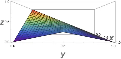
Unfortunately, $h$ is a little more complicated, as it is broken
up into cases. For $y\le\dfrac{1}{2}$, we have $h(x,y)=(1-y)(1-x)+\dfrac{y}{2}x$
(defined in 20). This means that as $x$ increases from
$0$ to $1$, $h$ interpolates linearly from $1-y\ge\dfrac{1}{2}$
to $\dfrac{y}{2}\le\dfrac{1}{4}$.And for $y\ge\dfrac{1}{2}$, the
coefficient of $x$ in $h$ changes to $\dfrac{1}{2}-\dfrac{y}{2}$
so that, as $x$ increases, $h$ interpolates linearly from $1-y\le\dfrac{1}{2}$
to $\dfrac{1}{2}-\dfrac{y}{2}\le\dfrac{1}{4}$. Putting these together,
we have that $h$ interpolates from the line $1-y$ to a ^-shaped
combination of two segments with maximum height $\dfrac{1}{4}$. We
can graph $z=h(x,y)$ with code like 21 to produce:
In our context, for $z\le\dfrac{1}{2}$, as $\varphi$ increases from
$0$ to $\pi$, $z+h\left(\dfrac{\varphi}{\pi},z\right)$ interpolates
from $z+1-z=1$ (regardless of $z$) to $z+\dfrac{z}{2}=\dfrac{3z}{2}\le\dfrac{3}{4}$.
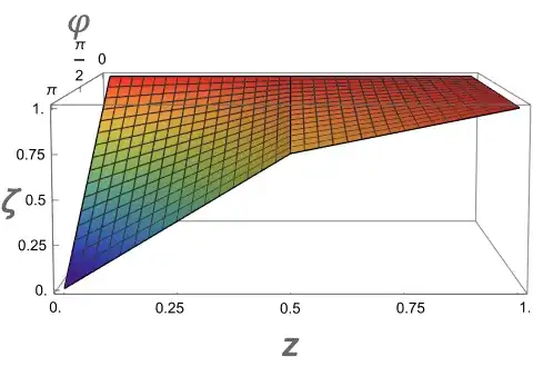
And for $z\ge\dfrac{1}{2}$, $z+h\left(\dfrac{\varphi}{\pi},z\right)$
interpolates from $1$ to $$z+\frac{1}{2}-\dfrac{z}{2}=\frac{z}{2}+\frac{1}{2}\boldsymbol{\ge}\frac{3}{4}.$$
Note that this means that for each $\varphi$ (except $0$), $\zeta=z+h\left(\dfrac{\varphi}{\pi},z\right)$
is an increasing function of $z$.
We can plot this with code like 22:
Case I: The inner part
Now that we have a sense for the individual component functions $\theta$
and $\zeta$ for the first case, we can put them together. $\theta$
has a range controlled by $z$ (not $\varphi$) that lengthens from
$\pi$ to $2\pi$ as $\varphi$ increases to $\pi$. And ignoring
the change in slope at $z=\dfrac{1}{2}$, $\zeta$ has a full range
at $z=0$ and the range shrinks towards the upper end as $z$ approaches
$1$.
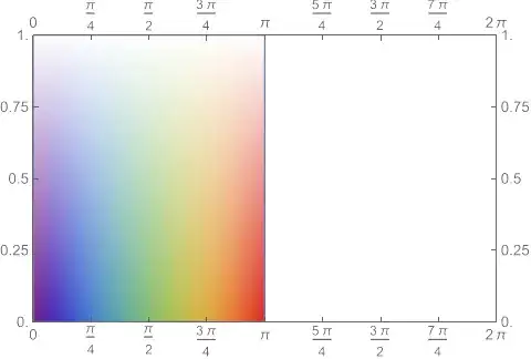
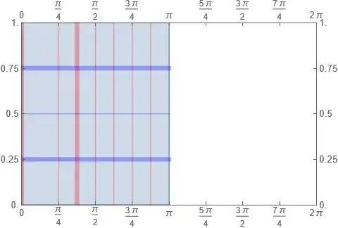
As before, we can see how $f$ reshapes the rectangle $\left[0,\pi\right]\times\left[0,1\right]$
using colors and carefully chosen gridlines. The domain for this case
looks like 23 or 24:
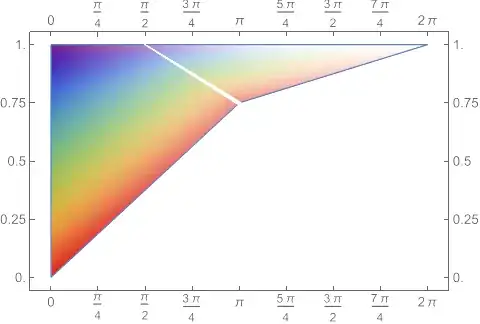
And $f$ transforms it by a sort of rotation and skew, as shown by
25 and 26:
Lastly, we can remind ourselves what the real subsets of the roll
$A_{2}$ look like. 27 and 28 produce:
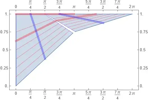
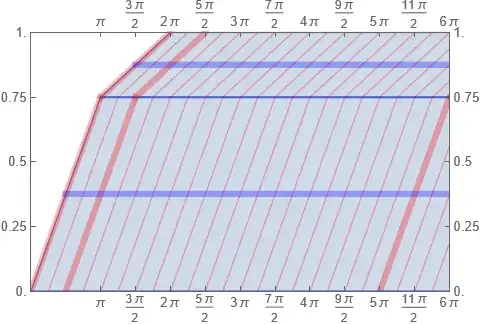
Cases II and III: The outer part
The rest of the strip in the input $\varphi z$-plane corresponding
to $\pi\le\varphi\le\infty$, $0\le z\le1$ is mapped by $f$ to some
region of the output plane via essentially the same map as was used
for the side:
$$(\varphi,z)\mapsto\begin{cases}
\left(\varphi+\pi(2z)-\pi,\frac{3}{4}(2z)\right) & \text{ for }0\le2z\le1\\
\left(\varphi+\pi(2z-1),\frac{3}{4}+\frac{1}{4}(2z-1)\right) & \text{ for }0\le2z-1\le1
\end{cases}\text{.}$$
We have the same slope/twist with a difference at $z=\dfrac{1}{2}$
corresponding to $\zeta=\dfrac{3}{4}$ as before. The difference here
is that the input and output angle parameters have infinite range.
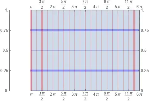
One way to look at this with gridlines (up to an arbitrary angle of
$6\pi$) might be this (29 and 30):
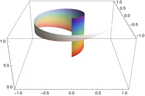
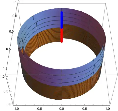
We can try to reproduce our success with the edge here with the roll,
but it does not look nearly as clear. 31 and 32 produce:

Continuity for the roll $A_{2}$
Continuity between cases II and III was already established for the
side $A_{3}$. And continuity between case I and the others can be
checked with a bit of algebra: $$z+h(1,z)=\begin{cases}
z+\frac{z}{2} & z\le\frac{1}{2}\\
z+\left(\frac{1}{2}-\frac{z}{2}\right) & z\ge\frac{1}{2}
\end{cases}$$ has essentially the same case distinction as case II vs. III. And
$\varphi=\pi$ means that
$$\varphi+\pi g\left(\frac{\varphi}{\pi},z\right)=\pi+\pi g(1,z)=\pi+\pi\left((-1)(1-z)+z\right)=2\pi z=\varphi-\pi+2\pi z$$
Continuity of $f$
$f$ nearly sends each piece to itself (except for the inner disk
of the domain mapping to a segment on the roll) in a way that is continuous
(we already verified the cases in the piecewise definitions). The
only remaining continuity issues to worry about are:
- Is $f$ well-defined on the intersection of the base $A_{1}$ and
the roll $A_{2}$?
- As the open base $A_{1}$ approaches the side $A_{3}$, does $f$
approach the correct values?
- As the roll $A_{2}$ approaches the side $A_{3}$, does $f$ on the
roll suitably approach the correct values on the side?
Issue 1: The Spiral Intersection
For the restriction of $f$ to the base $A_{1}$, we saw that $r_{0}=\dfrac{2}{\pi}\arctan\pi\approx0.8$
was a critical value where the behavior changed. So we may as well
split up the domain and verify that in each case the points in the
spiral intersection $A_{1}\cap A_{2}$ are mapped to the same points
by both definitions of $f$.
Case I: The Inner Spiral
Note that the spiral satisfies $r=\dfrac{2}{\pi}\arctan\varphi$ and
$r_{0}=\dfrac{2}{\pi}\arctan\pi$, so that $r\le r_{0}$ (for the
first case of the $A_{1}$ definition) is equivalent to $\varphi\le\pi$,
corresponding to the first case of the $A_{2}$ definition.
Under the $A_{1}$ definition, a point $\left(\dfrac{2}{\pi}\arctan\varphi,\varphi,0\right)$
(with $r\le r_{0}$) is sent to $$\left(0,0,1-\frac{\tan\left(\frac{\pi}{2}\left(\frac{2}{\pi}\arctan\varphi\right)\right)}{\pi}\right)=\left(0,0,1-\frac{\varphi}{\pi}\right)$$.
And under the $A_{2}$, definition, $\left(\dfrac{2}{\pi}\arctan\varphi,\varphi,0\right)$
(with $\varphi\le\pi$) is sent to
$$\left(\frac{2}{\pi}\arctan\left(\varphi+\pi g\left(\frac{\varphi}{\pi},0\right)\right),\varphi+\pi g\left(\frac{\varphi}{\pi},0\right),0+h\left(\frac{\varphi}{\pi},0\right)\right)$$
$$=\left(\frac{2}{\pi}\arctan\left(\varphi+\pi\left(-\frac{\varphi}{\pi}\right)\right),\varphi+\pi\left(-\frac{\varphi}{\pi}\right),1-\frac{\varphi}{\pi}\right)$$
$$=\left(\frac{2}{\pi}\arctan\left(0\right),0,1-\frac{\varphi}{\pi}\right)=\left(0,0,1-\frac{\varphi}{\pi}\right)\checkmark$$
Case II: The Outer Spiral
The other case has $\varphi\ge\pi$ so that $r\ge r_{0}$. Under the
$A_{1}$ definition, a point $\left(\dfrac{2}{\pi}\arctan\varphi,\varphi,0\right)$
(with $r\ge r_{0}$) is sent to $$\left(\frac{2}{\pi}\arctan\left(\tan\left(\frac{\pi}{2}\left(\frac{2}{\pi}\arctan\varphi\right)\right)-\pi\right),\varphi-\pi,0\right)=\left(\frac{2}{\pi}\arctan(\varphi-\pi),\varphi-\pi,0\right).$$
And under the $A_{2}$ definition, $\left(\dfrac{2}{\pi}\arctan\varphi,\varphi,0\right)$
(with $\varphi\ge\pi$) is sent to
$$\left(\frac{2}{\pi}\arctan(\varphi-\pi+2\pi0),\varphi-\pi+2\pi0,0+\frac{0}{2}\right)$$
$$=\left(\frac{2}{\pi}\arctan(\varphi-\pi),\varphi-\pi,0\right)\checkmark$$
Issue 2: The Bottom Edge
First, using the definition for the base $A_{1}$:
$$\lim_{r\to1^{-}}f\left(r,\varphi,0\right)$$
$$=\lim_{r\to1^{-}}\left(\frac{2}{\pi}\arctan\left(\tan\left(\frac{\pi}{2}r\right)-\pi\right),\varphi-\pi,0\right)\text{ since }1>r_{0}\approx0.8$$
$$=\left(\frac{2}{\pi}\arctan\infty,\varphi-\pi,0\right)=(1,\varphi-\pi,0)\text{.}$$
And then, using the definition for the side $A_{3}$: $f(1,\varphi,0)=\left(1,\varphi-\pi+2\pi0,0+\dfrac{0}{2}\right)=(1,\varphi-\pi,0)\checkmark$
Issue 3: Approaching the Side
Let $\varphi_{1}$ and $z_{1}$ be given. Then $$f\left(1,\varphi_{1},z_{1}\right)=\left(1,\theta_{1},\zeta_{1}\right):=\begin{cases}
\left(1,\varphi_{1}-\pi+2\pi z_{1},\frac{3}{2}z_{1}\right) & \text{ for }z_{1}\le\frac{1}{2}\\
\left(1,\varphi-\pi+2\pi z_{1},\frac{z_{1}+1}{2}\right) & \text{ for }z_{1}\ge\frac{1}{2}
\end{cases}.$$ Let $\varepsilon>0$ be given. Then an arbitrarily small neighborhood
in $A$ around $\left(1,\theta_{1},\zeta_{1}\right)$ is given by
the set of $\left(\rho,\theta,\zeta\right)$ such that $\rho>1-\varepsilon$,
$\left|\theta-\theta_{1}\right|\mod2\pi<\varepsilon$, $\left|\zeta-\zeta_{1}\right|<\varepsilon$.
The points on the side have been accounted for, so we just must show
that we can choose a neighborhood around $\left(1,\varphi_{1},z_{1}\right)$
so that the points on the roll in that neighborhood are mapped into
this $\varepsilon$-neighborhood. Firstly, we may safely assume $\varphi>\pi$
(by adding a multiple of $2\pi$ and hence taking a smaller neighborhood
of $\left(1,\varphi_{1},z_{1}\right)$ if needed). Therefore, $f$
is given by a function whose angle and height coordinates are identical
to the formulas for the side.
$$\left|\varphi-\pi+2\pi z-\left(\varphi_{1}-\pi+2\pi z_{1}\right)\right|$$
$$=\left|\varphi-\varphi_{1}+2\pi\left(z-z_{1}\right)\right|$$
$$\le\left|\varphi-\varphi_{1}\right|+2\pi\left|z-z_{1}\right|$$
To make sure this is less than $\varepsilon$, we may choose $\left|z-z_{1}\right|<\dfrac{\varepsilon}{4\pi}$
and $\left|\varphi-\varphi_{1}\right|<\dfrac{\varepsilon}{2}$. Then
note that we have $\left|z-z_{1}\right|<\dfrac{\varepsilon}{4\pi}<\dfrac{2}{3}\varepsilon$
so that $\left|\dfrac{3}{2}z-\dfrac{3}{2}z_{1}\right|<\varepsilon$
(handling the case of $z_{1}<\dfrac{1}{2}$) and $\left|\dfrac{z+1}{2}-\dfrac{z_{1}+1}{2}\right|<\dfrac{1}{3}\varepsilon<\varepsilon$
(handling the case of $z_{1}>\dfrac{1}{2}$). In the event that $z_{1}=\dfrac{1}{2}$
then $z$ may lie on either side of $z_{1}$, but this is fine because
$\dfrac{z_{1}+1}{2}=\dfrac{3}{2}z_{1}$ and we have both inequalities.
Finally, by adding a suitable multiple of $2\pi$ to $\varphi$, we
may ensure that $\varphi>\tan\left(\dfrac{\pi}{2}(1-\varepsilon)\right)$
so that $\rho=\dfrac{2}{\pi}\arctan(\varphi)>1-\varepsilon$.
Code Appendix
ar=AspectRatio
b=Blend
cf=ColorFunction
cfs=ColorFunctionScaling
e=Range
f=Function
ft=FrameTicks
gr=1/GoldenRatio
lb=LightBlue
lg=LightGray
ms=MeshStyle
n=False
pp=ParametricPlot
pps=PlotPoints
pp3=ParametricPlot3D
pr=PlotRange
ps=PlotStyle
rb=ColorData["Rainbow"]
st=Style
t=Thickness
u=Union
vp=ViewPoint
(*1*)Show[pp3[{r Cos[],r Sin[],0},{r,0,1},{,0,2π},vp->{0,-2,2},Mesh->n,pps->50],pp3[{Cos[],Sin[],z},{,0,2π},{z,0,1},vp->{0,-2,2},Mesh->n,pps->50]]
(*2*)PolarPlot[(2/π)ArcTan[],{,0,100π},pps->500]
(*3*)Show[pp3[{r Cos[],r Sin[],0},{r,0,1},{,0,2π},vp->{0,-2,2},Mesh->n,pps->50,ps->Yellow],pp3[{Cos[],Sin[],z},{,0,2π},{z,0,1},vp->{0,-2,2},Mesh->n,pps->50,ps->{Red,Opacity[.5]}],pp3[{(2/π)ArcTan[]Cos[],(2/π)ArcTan[]Sin[],z},{,0,6π},{z,0,1},vp->{0,-2,2},pps->50,ps->lb]]
(*4*)pp3[{Cos[],Sin[],z},{z,0,1/2},{,0,2π},pr->{{-1,1},{-1,1},{0,1}},Mesh->n,cf->f[{x,y,h,z,},b[{rb[/(2π)],lg},2z]],cfs->n,vp->{0,-2,1}]
(*5*)pp3[{Cos[-π+2π z],Sin[-π+2π z],(3/4)(2z)},{z,0,1/2},{,0,2π},pr->{{-1,1},{-1,1},{0,1}},Mesh->n,cf->f[{x,y,h,z,},b[{rb[/(2π)],lg},2z]],cfs->n,vp->{0,-2,1}]
(*6*)pp3[{Cos[],Sin[],z},{z,1/2,1},{,0,2π},pr->{{-1,1},{-1,1},{0,1}},Mesh->n,cf->f[{x,y,h,z,},b[{rb[/(2π)],lg},2z-1]],cfs->n,vp->{0,-2,1}]
(*7*)pp3[{Cos[-π+2π z],Sin[-π+2π z],(z+1)/2},{z,1/2,1},{,0,2π},pr->{{-1,1},{-1,1},{0,1}},Mesh->n,cf->f[{x,y,h,z,},b[{rb[/(2π)],lg},2z-1]],cfs->n,vp->{0,-2,1}]
(*8*)Show[pp3[{Cos[],Sin[],z},{z,0,1/2},{,0,2π},Mesh->{e[.001,1/2,1/24],u[{{.001,{Red,t[.02]}}},e[.001+π/4,2π,π/4]]}],pp3[{Cos[],Sin[],z},{z,1/2,1},{,0,2π},ps->lb,Mesh->{e[1/2+.001,1,1/8],u[{{.001,{Blue,t[.02]}}},e[.001+π/4,2π,π/4]]}],pr->All,vp->{2,0,1.5}]
(*9*)Show[pp3[{Cos[-π+2π z],Sin[-π+2π z],(3/4)(2z)},{z,0,1/2},{,0,2π},Mesh->{e[.001,1/2,1/24],u[{{.001,{Red,t[.02]}}},e[.001+π/4,2π,π/4]]}],pp3[{Cos[-π+2π z],Sin[-π+2π z],(z+1)/2},{z,1/2,1},{,0,2π},ps->lb,Mesh->{e[1/2+.001,1,1/8],u[{{.001,{Blue,t[.02]}}},e[.001+π/4,2π,π/4]]}],pr->All,vp->{2,0,1.5}]
(*10*)r0=2ArcTan[π]/π
(*11*)Plot[(2/π)ArcTan[Tan[π r/2]-π],{r,r0,1}]
(*12*)pp[{r Cos[],r Sin[]},{r,r0,1},{,0,2π},Mesh->n,pps->20,cf->f[{x,y,r,},b[{rb[/(2π)],White},(r-r0)/(1-r0)]],cfs->n]
(*13*)pp[{(2/π)ArcTan[Tan[π r/2]-π]Cos[-π],(2/π)ArcTan[Tan[π r/2]-π]Sin[-π]},{r,r0,1},{,0,2π},Mesh->n,pps->20,cf->f[{x,y,r,},b[{rb[/(2π)],White},(r-r0)/(1-r0)]],cfs->n]
(*14*)Plot[1-Tan[π r/2]/π,{r,0,r0}]
(*15*)pp[{r Cos[],r Sin[]},{r,0,r0},{,0,2π},Mesh->n,pps->20,cf->f[{x,y,r,},b[{Black,lg},r/r0]],cfs->n]
(*16*)pp3[{0,0,1-Tan[π r/2]/π},{r,0,r0},Mesh->n,pps->20,cf->f[{x,y,z,r},b[{Black,lg},r/r0]],cfs->n,vp->{0,-2,.5},ps->t[.05]]
(*17*)g[x_,y_]:=(-x)(1-y)+y
(*18*)Plot3D[g[x,y],{x,0,1},{y,0,1},cf->f[{x,y,z},rb[z]],AxesLabel->{st[x,Large,Bold],st[y,Large,Bold],st[z,Large,Bold]},vp->Front,pr->All]
(*19*)Plot3D[+π g[/π,z],{,0,π},{z,0,1},cf->f[{,z,θ},rb[θ]],AxesLabel->{st[,Large,Bold],st[z,Large,Bold],st[θ,Large,Bold]},vp->Front,pr->All,Ticks->{e[0,π,π/4],e[0,1,1/4],e[0,2π,π/2]}]
(*20*)h[x_,y_]:=(1-y)(1-x)+Piecewise[{{y,y<=1/2},{1-y,y>=1/2}}]x/2
(*21*)Show[Plot3D[h[x,y],{x,0,1},{y,0,1/2},cf->f[{x,y,z},rb[z]]],Plot3D[h[x,y],{x,0,1},{y,1/2,1},cf->f[{x,y,z},rb[z]],cfs->n],AxesLabel->{st[x,Large,Bold],st[y,Large,Bold],st[z,Large,Bold]},vp->Right,pr->All]
(*22*)Show[Plot3D[z+h[/π,z],{,0,π},{z,0,1/2},cf->f[{,z,ζ},rb[ζ]]],Plot3D[z+h[/π,z],{,0,π},{z,1/2,1},cf->f[{,z,ζ},rb[ζ]],cfs->n],AxesLabel->{st[,Large,Bold],st[z,Large,Bold],st[ζ,Large,Bold]},vp->{4,0,.5},pr->All,Ticks->{e[0,π,π/2],e[0,1,.25],e[0,1,.25]}]
(*23*)pp[{,z},{,0,π},{z,0,1},cf->f[{x,y,,z},b[{rb[],White},z]],ft->{e[0,2π,π/4],e[0,1,.25]},pr->{{0,2π},{0,1}},ar->gr]
(*24*)pp[{,z},{,0,π},{z,0,1},ft->{e[0,2π,π/4],e[0,1,.25]},pr->{{0,2π},{0,1}},ar->gr,Mesh->{u[{{.001,{Red,t[.015]}},π/4+.001,{3π/8+.001,{Red,t[.015]}}},e[.001+π/2,π,π/8]],{.001,{1/4+.001,{Blue,t[.015]}},1/2+.001,{3/4+.001,{Blue,t[.015]}}}},ms->{Red,Blue}]
(*25*)Show[pp[{+π g[/π,z],z+h[/π,z]},{,0,π},{z,0,1/2},cf->f[{x,y,,z},b[{rb[/π],White},z]],cfs->n,pps->50],pp[{+π g[/π,z],z+h[/π,z]},{,0,π},{z,1/2,1},cf->f[{x,y,,z},b[{rb[/π],White},z]],cfs->n,pps->50],ft->{e[0,2π,π/4],e[0,1,.25]},pr->{{0,2π},{0,1}},ar->gr]
(*26*)Show[pp[{+π g[/π,z],z+h[/π,z]},{,0,π},{z,0,1/2},Mesh->{u[{{.001,{Red,t[.015]}},π/4+.001,{3π/8+.001,{Red,t[.015]}}},e[.001+π/2,π,π/8]],{.001,{1/4+.001,{Blue,t[.015]}},1/2-.01}},ms->{Red,Blue}],pp[{+π g[/π,z],z+h[/π,z]},{,0,π},{z,1/2,1},Mesh->{u[{{.001,{Red,t[.015]}},π/4+.001,{3π/8+.001,{Red,t[.015]}}},e[.001+π/2,π,π/8]],{1/2+.01,{3/4+.001,{Blue,t[.015]}}}},ms->{Red,Blue}],ft->{e[0,2π,π/4],e[0,1,.25]},pr->Full,ar->gr]
(*27*)pp3[{(2/π)ArcTan[]Cos[],(2/π)ArcTan[]Sin[],z},{,0,π},{z,0,1},cf->f[{x,y,h,,z},b[{rb[],White},z]],pps->20,Mesh->None,pr->{{-1,1},{-1,1},{0,1}},vp->{0,-2,1}]
(*28*)Show[pp3[{(2/π)ArcTan[+π g[/π,z]]Cos[+π g[/π,z]],(2/π)ArcTan[+π g[/π,z]]Sin[+π g[/π,z]],z+h[/π,z]},{,0,π},{z,0,1/2},cf->f[{x,y,h,,z},b[{rb[/π],White},z]],cfs->n,pps->20,Mesh->None],pp3[{(2/π)ArcTan[+π g[/π,z]]Cos[+π g[/π,z]],(2/π)ArcTan[+π g[/π,z]]Sin[+π g[/π,z]],z+h[/π,z]},{,0,π},{z,1/2,1},cf->f[{x,y,h,,z},b[{rb[/π],White},z]],cfs->n,pps->20,Mesh->None],pr->{{-1,1},{-1,1},{0,1}},vp->{0,-2,1}]
(*29*)pp[{,z},{,π,6π},{z,0,1},ft->{e[π,6π,π/2],e[0,1,.25]},pr->{{0,6π},{0,1}},ar->gr,Mesh->{u[{{π+.001,{Red,t[.015]}},5π/4+.001,{3π/2+.001,{Red,t[.015]}}},e[.001+7π/4,23π/4,π/4],{{23π/4+.001,{Red,t[.015]}}}],{.001,{1/4+.001,{Blue,t[.015]}},1/2+.001,{3/4+.001,{Blue,t[.015]}}}},ms->{Red,Blue}]
(*30*)Show[pp[{-π+2π z,3z/2},{,π,7π},{z,0,1/2},ft->{e[π,6π,π/2],e[0,1,.25]},pr->{{0,6π},{0,1}},ar->gr,Mesh->{u[{{π+.001,{Red,t[.015]}},5π/4+.001,{3π/2+.001,{Red,t[.015]}}},e[.001+7π/4,23π/4,π/4],{{23π/4+.001,{Red,t[.015]}}},e[.001+23π/4,7π,π/4]],{.001,{1/4+.001,{Blue,t[.015]}},1/2-.002}},pps->50,ms->{Red,Blue}],pp[{-π+2π z,(z+1)/2},{,π,7π},{z,1/2,1},ft->{e[π,6π,π/2],e[0,1,.25]},pr->{{0,6π},{0,1}},ar->gr,Mesh->{u[{{π+.001,{Red,t[.015]}},5π/4+.001,{3π/2+.001,{Red,t[.015]}}},e[.001+7π/4,23π/4,π/4],{{23π/4+.001,{Red,t[.015]}}},e[.001+23π/4,7π,π/4]],{1/2+.002,{3/4+.001,{Blue,t[.015]}}}},pps->50,ms->{Red,Blue}]]
(*31*)Show[pp3[{(2/π)ArcTan[]Cos[],(2/π)ArcTan[]Sin[],z},{,π,6π},{z,0,1/2},Mesh->{u[{{.001+π,{Red,t[.02]}}},e[.001+5π/4,6π,π/4]],e[.001,1/2,1/24]},pps->30],pp3[{(2/π)ArcTan[]Cos[],(2/π)ArcTan[]Sin[],z},{,π,6π},{z,1/2,1},ps->lb,Mesh->{u[{{.001+π,{Blue,t[.02]}}},e[.001+5π/4,6π,π/4]],e[1/2+.001,1,1/8]},pps->30],pr->All,vp->{2,0,2.25}]
(*32*)Show[pp3[{(2/π)ArcTan[-π+2π z]Cos[-π+2π z],(2/π)ArcTan[-π+2π z]Sin[-π+2π z],3z/2},{,π,6π},{z,0,1/2},Mesh->{u[{{.001+π,{Red,t[.02]}}},e[.001+5π/4,6π,π/4]],e[.001,1/2,1/24]},pps->30],pp3[{(2/π)ArcTan[-π+2π z]Cos[-π+2π z],(2/π)ArcTan[-π+2π z]Sin[-π+2π z],(z+1)/2},{,π,6π},{z,1/2,1},ps->lb,Mesh->{u[{{.001+π,{Blue,t[.02]}}},e[.001+5π/4,6π,π/4]],e[1/2+.001,1,1/8]},pps->30],pr->All,vp->{2,0,2.25}]


