Why do the roots of $\int_0^x (1-s^2)^n ds$ lie on a lemniscate?

Question

Consider the polynomial $$f_n(x)=\int_0^x (1-s^2)^n ds$$ for some integer $n$. I am interested in these polynomials for reasons unrelated to this question: these are the odd polynomials of which the maximum possible number of derivatives vanish at $x=\pm 1$.

The first few such polynomials are $$f_0(x)=x$$ $$f_1(x)=x-\frac{x^3}{3}$$ $$f_2(x)=x-\frac{2 x^3}{3}+\frac{x^5}{5}$$ $$f_3(x)=x-x^3+\frac{3 x^5}{5}-\frac{x^7}{7}$$

On a whim, I plotted the roots of these polynomials, I find that they all lie on a lemniscate. For example, for $n=50$,

I suspect there is some "limit lemniscate" as $n\rightarrow \infty$. This comes as a complete surprise to me. Why should the roots of these polynomials lie on a lemniscate, at all?

Answer 1

Fig. 1 : The roots of polynomial $f_{31}$ and the standard lemniscate with equ. $(x^2+y^2)^2=2(x^2-y^2)$. This figure has been drawn with a "SAGE" program (see remark at the bottom).

The remarkable last comments by @Semiclassical

$$\begin{cases}f_n(Z)&=&{_2}F_{1}(1/2,-n;3/2,Z^2)\color{red}{Z}\\ f_n(\sqrt{1-z})&=&{_2}F_{1}(1/2,-n;3/2,1+z)\color{red}{\sqrt{1-z}}\end{cases}$$

can be understood at the light of the following

Lemma : the (double) complex mapping defined by :

$$z \mapsto Z=\pm \sqrt{1+z} \ \iff \ Z^2=1+z\tag{1}$$

maps the unit circle $U$ onto the "unit lemniscate".

Proof of lemma : (1) is equivalent to

$$(Z-1)(Z+1)=z$$

Therefore, we have :

$$|Z-1| |Z+1|=|z|$$

As a consequence, constraining $z$ to be with modulus $1$ is equivalent to say that the product of distances of $Z$ to "foci" $-1$ and $+1$ is equal to constant $1$, which is one of the definitions of Bernoulli's lemniscate, as a particular case of Cassini ovals). $\square$

Fig. 2.

Now, it remains to establish that the roots of the second polynomial in (1) are closer and closer to the unit circle $U$ as examplified by figure 3 obtained using Wolfram Alpha (see Remark 3 below) in the case $n=15$ : not only are they close to $U$ but also close to the $n+1=16$th roots of unity. Therefore, the question remains open...

Fig. 3.

Remarks :

1. Fig. 1 has been drawn with the following "SAGE" program :

    from sage.functions.hypergeometric import closed_form
    var('x y')
    P = lambda n : simplify(closed_form(hypergeometric([1/2,-n],[3/2], x^2)))
    g=Graphics()
    L=[[0,0]]
    w=P(32)
    s=w.roots(ring=CDF)
    for k in range(len(s)) :
       u=s[k][0]
       L.append([real_part(u),imag_part(u)])
    g+=plot(point(L,color='red', xmin=-2,xmax=2, ymin = -1, ymax = 1, aspect_ratio=1))
    g+=implicit_plot((x^2+y^2)^2==2*(x^2-y^2),(x,-2,2),(y,-1,1))
    g+=plot(line(([-2,0],[2,0]),color='black'))
    g+=plot(line(([0,-1],[0,1]),color='black'))
    show(g)
   

2. Fig. 2 has been drawn using the following Matlab script :

    t=0:pi/100:2*pi;
    plot(1+exp(i*t));hold on;axis equal;
    for s=-1:2:1
       plot(s*sqrt(1+exp(i*t)));hold on;
    end;
   

3. Fig. 3 has been obtained with Wolfram Alpha by asking :

$$\text{roots (sqrt(1+x) 2F1(1/2, -15, 3/2, 1+x))}$$

Answer 2

Definitions: Let $p_n(z)=(1-z^2)^n$. Now fix $n\geq1$ and let $p=p_n$, $f=f_n$, $x_0=0$ and let $x_+$ be the positive root if $n$ is odd and if $n$ is even define $x_+$ to be the unique positive real such that $\vert f(x_+)\vert=2\vert f(1)\vert$ and for $i\geq1$ let $x_i$ be the remaining roots in the right half plane (because of the symmetry over the imaginary axis it is enough to show the claim for these zeros). We will use $x$ to denote any of these zeros. Further define the filled level sets $S_h=\{z:\vert1-z^2\vert\leq h\}$. For a curve $\gamma:[0,\infty)\to\mathbb{C}$ define the curve $\tilde\gamma:[0,\infty)\to\mathbb{R}^2$ with $\tilde\gamma(h)=(\Re(\gamma(h)),\Im(\gamma(h)))$. Further set $\gamma_+=\gamma_{x_+}$ and $\gamma_0=\gamma_{x_0}$.

We will make use of $\nabla_{x,y}$ which is the gradient, for example $\nabla_{x,y}\vert(1-(x+iy)^2)\vert\big\vert_{x+iy=\gamma_x(h)}$ means the gradient of the real function $\vert(1-(x+iy)^2)\vert$ with respect to $(x,y)$ evaluated at $x=\Re(\gamma_x(h))$ and $y=\Im(\gamma_x(h))$.

Note that for any level set $L=\{z:\vert1-z^2\vert= h\}$ we have for all $z\in L$ that $z_0\leq\vert z\vert\leq z_+$ where $z_0$ is, if it exists (i.e. if $h\leq1$), is the smaller point of the intersection of $L$ with the non negative real axis and $z_+$ is the bigger one (either see it by the forumla $\vert1-z^2\vert=h$ or transform this formula into polar coordinates).

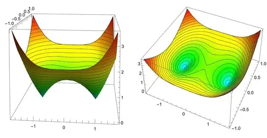
We will use the variables $h$ and $H$ which stand for height. If $z\in\mathbb{C}$ the height of $z$ is $\vert 1-z^2\vert$. Here is a picture of the surface (seen from two different angles) parametrized by $\vert 1-(x+i y)^2\vert$ where the colors represent the height and the lines drawn on the surface are the level sets.

Strategy of proof:

We will squeeze the zeros between two level sets:

Below we will define curves $\gamma_x$ with $\gamma_x(0)=1$ which go through $x$ such that $\vert1-\gamma_x(h)^2\vert=h$ (this just means that $\gamma_x(h)$ is parametrized by height, so $\gamma_x(h)$ has height $h$). So we get for $\gamma_x(H)=Z$ (so $\vert 1-Z^2\vert=H$) that

$$f_n(Z)=\int_0^Zp_n(z)dz=\int_0^1p_n(z)dz+\int_1^Zp_n(z)dz=f_n(1)+\int\limits_{\gamma_x\big\vert_{[0,H]}}p_n(z)dz$$

so it is enough to show, since $f_n(1)$ is a non zero real, that

$$\left\vert\int\limits_{\gamma_+\big\vert_{[0,H]}}p_n(z)dz\right\vert\leq\left\vert\int\limits_{\gamma_x\big\vert_{[0,H]}}p_n(z)dz\right\vert\leq\left\vert\int\limits_{\gamma_0\big\vert_{[0,H]}}p_n(z)dz\right\vert$$

where $\gamma_0$ and $\gamma_+$ are the curves on the real line (the right inequality holds up to $H=1$, the left holds for $H\geq0$). This chain of inequalites implies

$$\operatorname{height}x_0\leq\operatorname{height}x\leq\operatorname{height}x_+.$$

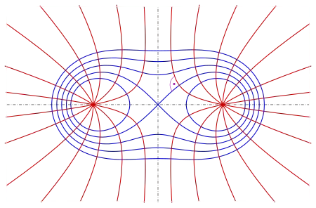
Intuition: The intuition for what's going on in the following is just this: The level sets are densest on the real axis to the right of $1$ and sparsest on the real axis to the left of $1$ (up to $0$) and the density is $\Vert\nabla_{x,y}\vert p(x+iy)\vert\Vert$.

Proof

Claim: The polynomial $f$ hasn't got any non zero zeros inside $S_1$. For this define for each $x$ the unique curve $\gamma_x:[0,\infty)\to\mathbb{C}$ (except for $x_0$ for which the domain is $[0,1]$) with the following properties:

1. $\tilde\gamma_x'(h)$ is parallel to $\nabla_{x,y}\vert(1-(x+iy)^2)\vert\big\vert_{x+iy=\gamma_x(h)}$ (orthogonal trajectory)

2. $\vert (1-\gamma_x(h)^2)\vert=h$ (choice of parametrization - parametrization by height)

3. $\gamma_x(0)=1$ (choice of initial point)

4. $\gamma_x(\vert1-\gamma_x(x)^2\vert)=x$ (choice of initial angle - $\gamma_x$ goes through $x$)

We have

$$\vert p(\gamma_x(h))\vert=h^n$$

so

$$\Vert\nabla_{x,y}\vert p(x+iy)\vert\big\vert_{x+iy=\gamma_x(h)}\Vert\vert\gamma_x^{'}(h)\vert=\nabla_{x,y}\vert p(x+iy)\vert\big\vert_{x+iy=\gamma_x(h)}\cdot\tilde\gamma_x^{'}(h)=\vert p(\gamma_x(h))\vert^{'}=nh^{n-1}$$

hence

$$\vert\gamma_x^{'}(h)\vert=\frac{nh^{n-1}}{\Vert\nabla_{x,y}\vert p(x+iy)\vert\big\vert_{x+iy=\gamma_x(h)}\Vert}=\frac{nh^{n-1}}{\vert p'(\gamma_x(h))\vert}=\frac{nh^{n-1}}{\vert-2\gamma_x(h)n(1-\gamma(h)^2)^{n-1}\vert}=$$

$$\frac{h^{n-1}}{\vert2\gamma_x(h)h^{n-1}\vert}=\frac{1}{2\vert\gamma_x(h)\vert}$$

therefore

$$\left\vert\int\limits_{\gamma_x\big\vert_{[0,H]}}p(z)dz\right\vert=\left\vert\int\limits_0^Hp(\gamma_x(h))\gamma_x^{'}(h)dh\right\vert\leq\int\limits_0^H\vert p(\gamma_x(h))\gamma_x^{'}(h)\vert dh=\int\limits_0^Hh^n\vert\gamma_x^{'}(h)\vert dh=$$

$$\int\limits_0^Hh^n\vert\gamma_x^{'}(h)\vert dh=\int\limits_0^H\frac{h^n}{2\vert\gamma_x(h)\vert} dh\leq\int\limits_0^H\frac{h^n}{2\gamma_0(h)} dh=\left\vert\int\limits_0^Hh^n\gamma_0(h)^{'} dh\right\vert=\left\vert\int\limits_{\gamma_0\big\vert_{[0,H]}}p(z)dz\right\vert$$

which establishes the claim.

Claim: All roots of $f$ are contained in $S_{\vert 1-x_+^2\vert}$. For this define for each $x$ the unique curve $\gamma_x:[0,\infty)\to\mathbb{C}$ (except for $x_0$ for which the domain is $[0,1]$) with the following properties:

1. $\forall h\geq0\text{ }f(\gamma_x(h))\in\mathbb{R}$ (line of constant argument of $f$)

2. $\vert (1-\gamma_x(h)^2)\vert=h$ (choice of parametrization - parametrization by height)

3. $\gamma_x(0)=1$ (choice of initial point)

4. $\gamma_x(\vert1-\gamma_x(x)^2\vert)=x$ (choice of initial angle - $\gamma_x$ goes through $x$)

We have

$$\vert p(\gamma_x(h))\vert=h^n$$

so

$$\Vert\nabla_{x,y}\vert p(x+iy)\vert\big\vert_{x+iy=\gamma_x(h)}\Vert\vert\gamma_x^{'}(h)\vert\vert\cos\theta_x(h)\vert=\nabla_{x,y}\vert p(x+iy)\vert\big\vert_{x+iy=\gamma_x(h)}\cdot\tilde\gamma_x^{'}(h)=$$

$$\vert p(\gamma_x(h))\vert^{'}=nh^{n-1}$$

where $\theta_x(h)$ is the angle between the two quantities from which we took the dot product hence by a similar calculation as above

$$\vert\gamma_x^{'}(h)\vert=\frac{1}{2\vert\gamma_x(h)\vert\vert\cos\theta_x(h)\vert}$$

therefore

$$\left\vert\int\limits_{\gamma_+\big\vert_{[0,H]}}p(z)dz\right\vert=\left\vert\int\limits_0^Hp(\gamma_+(h))\gamma_+^{'}(h)dh\right\vert=\left\vert\int\limits_0^H\frac{h^n}{2\gamma_+(h)}dh\right\vert\leq\int\limits_0^H\left\vert\frac{h^n}{2\gamma_x(h)\cos\theta_x(h)}\right\vert dh=$$

$$\int\limits_0^H\left\vert\frac{p(\gamma_x(h))}{2\gamma_x(h)\cos\theta_x(h)}\right\vert dh=\left\vert\int\limits_0^Hp(\gamma_x(h))\gamma_x(h)^{'} dh\right\vert=\left\vert\int\limits_{\gamma_x\big\vert_{[0,H]}}p(z)dz\right\vert$$ where we used that $p(\gamma_x(h))\gamma_x(h)^{'}$ is real and of constant sign in the second last equality which establishes the claim.

Now clearly $\vert1-x_+^2\vert\to1$ as $n\to\infty$ and we are done.

Existence of solutions to differential equations: One can pick ones favorite local existence theorem. It is not hard, in this example, to show the existence and uniqueness of global solutions by hand by piecing together the local solutions.

There is one minor justification left to be done.

fedjafan

Answer 3

The Euler formula gives $$_2F_1(1/2,-n;3/2,1-z)=\frac{1}{2}\int_0^1(1-x+xz)^n\frac{dx}{\sqrt{x}}$$ which tends to zero when $|z|=1$ and $z\neq 1$ by dominated convergence.