I will use my answer to Newton method to solve nonlinear system as a guide and you can see another example using this method.
The regular Newton-Raphson method is initialized with a starting point $x_0$ and then you iterate $\tag 1x_{n+1}=x_n-\dfrac{f(x_n)}{f'(x_n)}$
In higher dimensions, there is an exact analog. We define:
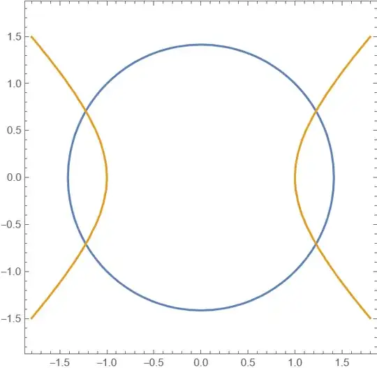
$$F\left(\begin{bmatrix}x_1\\x_2\end{bmatrix}\right) = \begin{bmatrix}f_1(x_1,x_2) \\ f_2(x_1,x_2) \end{bmatrix} = \begin{bmatrix}x_1^2 + x_2^2-2 \\ x_1^2-x_2^2 -1 \end{bmatrix} = \begin{bmatrix}0\\0\end{bmatrix}$$
The derivative of this system is the $2x2$ Jacobian given by:
$$J(x_1,x_2) = \begin{bmatrix} \dfrac{\partial f_1}{\partial x_1} & \dfrac{\partial f_1}{\partial x_2} \\ \dfrac{\partial f_2}{\partial x_1} & \dfrac{\partial f_2}{\partial x_2} \end{bmatrix} = \begin{bmatrix} 2x_1 & 2 x_2\\ 2 x_1 & -2x_2\end{bmatrix}$$
The function $G$ is defined as:
$$G(x) = x - J(x)^{-1}F(x)$$
and the functional Newton-Raphson method for nonlinear systems is given by the iteration procedure that evolves from selecting an initial $x^{(0)}$ and generating for $k \ge 1$ (compare this to $(1)$),
$$x^{(k)} = G(x^{(k-1)}) = x^{(k-1)} - J(x^{(k-1)})^{-1}F(x^{(k-1)}).$$
We can write this as:
$$\begin{bmatrix}x_1^{(k)}\\x_2^{(k)}\end{bmatrix} = \begin{bmatrix}x_1^{(k-1)}\\x_2^{(k-1)}\end{bmatrix} + \begin{bmatrix}y_1^{(k-1)}\\y_2^{(k-1)}\end{bmatrix}$$
where:
$$\begin{bmatrix}y_1^{(k-1)}\\y_2^{(k-1)}\end{bmatrix}= -\left(J\left(x_1^{(k-1)},x_2^{(k-1)}\right)\right)^{-1}F\left(x_1^{(k-1)},x_2^{(k-1)}\right)$$
Here is a starting vector:
$$x^{(0)} = \begin{bmatrix}x_1^{(0)}\\x_2^{(0)}\end{bmatrix} = \begin{bmatrix}1.5\\1.5\end{bmatrix}$$
You should end up with a solution that looks something like (you can do the iteration formula steps as it converges very quickly):
$$\begin{bmatrix}x_1\\x_2\end{bmatrix} = \begin{bmatrix} 1.22474\\0.707107\end{bmatrix}$$
As another example, I chose the following starting point
$$x^{(0)} = \begin{bmatrix}x_1^{(0)}\\x_2^{(0)}\end{bmatrix} = \begin{bmatrix}-150.\\150.\end{bmatrix}$$
The iterates still converged pretty quickly and these initial choices were way outside the actual roots (we do not always have such luck - see update below) as
$$\{-150.,150.\},\{-75.005,75.0017\},\{-37.5125,37.5042\},\{-18.7762,18.7587\},\{-9.42807,9.3927\},\{-4.79358,4.72297\},\{-2.55325,2.41442\},\{-1.57037,1.31075\},\{-1.26278,0.846107\},\{-1.22532,0.718524\},\{-1.22475,0.707197\},\{-1.22474,0.707107\},\{-1.22474,0.707107\}$$
Of course, for a different starting vector you are going to get a different solution and perhaps no solution at all.
For comparison, the four exact roots are
$$\left(x=-\sqrt{\frac{3}{2}}\land \left(y=-\frac{1}{\sqrt{2}}\lor y=\frac{1}{\sqrt{2}}\right)\right)\lor \left(x=\sqrt{\frac{3}{2}}\land \left(y=-\frac{1}{\sqrt{2}}\lor y=\frac{1}{\sqrt{2}}\right)\right)$$
Update What are approaches to choosing starting points?
Typically, you just choose a point at random. You could also use a contour plot and see if there are points of intersection as a guide in selecting the starting points (it depicts the four points of intersection, that is, the roots).
Sometimes, when solving nonlinear equations, coming up with a good initial guess is a bit of an art, that often requires some problem-specific understanding. If you start too far from a root, Newton’s method can sometimes take a large step, far outside the validity of the Taylor approximation, and this can actually make the guess worse. You can read some additional thoughts at How to choose an initial value for a multidimensional equation while using Newton-Raphson method to solve it?.
Convergence for the multidimensional Newton’s method is also quadratic (under some assumptions similar to those in the one-dimensional case), but the same and other issues can occur. You can see a proof and some comments at Prove or disprove - Newton's method convergence in higher dimensions.
