Orthogonal trajectories to family of curves $\left\Vert x \right\Vert_p=1$ where $x\in\mathbb{R}^2$

Question

I have been trying to find the orthogonal trajectories of the family of $p$-norm curves $\left\Vert x \right\Vert_p=1$, where $x\in\mathbb{R}^2$ and $p>0$. I eventually reached a step where I must find $p(x,y)$ such that $(1-x^{p(x,y)})^\frac{1}{p(x,y)}=y$ for all $x,y\in(0,1)$.

Does a closed-form expression for $p(x,y)$ exist? Graphing the equation with $p$ on the $z$ axis in a 3D graphing calculator at least suggests that $p$ is injective.

More importantly, is this not a good approach for finding the orthogonal trajectories? I am following the steps described in Find the orthogonal trajectories of the family of curves.

Answer 1

I think this is pretty much hopeless. I prefer to work implicitly.

We have a curve $(x(p),y(p))$ of points starting at $(x(p_0),y(p_0))=(x_0,y_0)$ and satisfying $$x(p)^p + y(p)^p=1 \quad\text{for all } p \text{ near } p_0.$$ As $p$ varies, we first want the tangent vector to this curve, so we differentiate with respect to $p$: Dropping the "$(p)$" for convenience, $$x^p\log x + px^{p-1}x'(p) + y^p\log y + py^{p-1}y'(p) = 0.$$ So the tangent vector to this curve has slope \begin{align*} \frac{y'(p)}{x'(p)} &= -\frac{x^p\log x+y^p\log y+px^{p-1}x'(p)}{py^{p-1} x'(p)}=-\left(\frac{x^p\log x+y^p\log y}{py^{p-1}x'(p)}+\left(\frac xy\right)^{p-1}\right)\\ &=-\left(\frac{x^p\log(\frac xy)+\log y}{py^{p-1}x'(p)}+\left(\frac xy\right)^{p-1}\right). \end{align*} This looks strange enough, as we have a very non-homogeneous factor of $x'$. Let's arbitrarily set $x'=1$. To find the orthogonal trajectory to the family of curves with these slopes we need the negative reciprocal slope, and so we need to solve $$\frac{dy}{dx} = \frac 1{\frac{x^p\log(\frac xy)+\log y}{py^{p-1}}+\left(\frac xy\right)^{p-1}},$$ remembering the constraint $x^p+y^p=1$. Good luck with that! (Time for a numerical solution.)

Answer 2

Let us give the name $(C_p)$ $(p>0)$ to the curve with implicit equation : $$|x|^p+|y|^p=1 \tag{1}$$

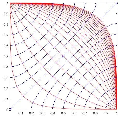
Fig. 1 : (some) curves $(C_p)$ in red. (Some of) their orthogonal curves in blue.

Due to the symmetry of curves $(C_p)$ with respect to coordinate axes, our study can be restricted to the square $(S):=(0,1)^2$, allowing to drop the $|...|$ symbols.

Important remark : curves $(C_p)$ provide a foliation of square $(S)$, i.e., that for each $(a,b) \in (S)$ there exists a unique $p=p(a,b)$ such that $a^p+b^p=1$.

We are going to work on

1. the following parametric representation of curves $(C_p)$ :

$$\begin{cases}x&=&x(t)&=&(\cos t)^{(2/p)}\\y&=&y(t)&=&(\sin t)^{(2/p)}\end{cases} \ \ (0 \le t \le \pi/2)$$

2. with a numerical approach combining a Runge-Kutta ODE solver (implemented in Matlab ; see program below) and Newton's method.

The tangent vector to $(C_p)$ in point $(x(t),y(t))$ is :

$$\begin{cases}x'(t)&=&\frac{2}{p}(\cos t)^{(2/p-1)}(-\sin t)&=&-\frac{2}{p}x(t) \tan t\\y'(t)&=&\frac{2}{p}(\sin t)^{(2/p-1)}\cos t&=& \ \ \ \frac{2}{p}y(t)\frac{1}{\tan t}\end{cases} \tag{2}$$

Orthogonal trajectories are obtained by replacing in (2)

$$\pmatrix{x'\\y'} \ \text{by} \ \pmatrix{\ \ y'\\-x'}$$

which means that the current point $(X,Y)$ is a solution to the following differential system :

$$\begin{cases}X'&=&\frac{2}{p}Y\frac{1}{\tan t}\\Y'&=&\frac{2}{p}X \tan t\end{cases}\tag{3}$$

We can get rid of common factor $\frac{2}{p}$, giving the simpler system :

$$\begin{cases}X'&=&Y\frac{1}{\tan t}\\Y'&=&X \tan t\end{cases}\tag{4}$$

System (4) cannot be given "as such" to an ODE solver. We need for that to express $t$ (and in fact $p$ as well) as functions of $X$ and $Y$ :

• for $t$, we use relationships :

$$\begin{cases}x&=&(\cos t)^{2/p}\\1 + (\tan t)^2 &=& \frac{1}{(\cos t)^2} \end{cases} \ \ \text{giving} \ \ \tan t = \sqrt{\tfrac{1}{x^p}-1}$$

• for $p$ : being given a point with coordinates $(a,b)$ in square $(S)$, how can we "output" the unique value of $p$ such that : $a^p+b^p=1$ (according to the "foliation" principle) ? By using Newton's algorithm, i.e., with the recurrence relationship :

$$p_{n+1}=p_n - \frac{f(p_n)}{f'(p_n)}$$

where $f(x):=a^x+b^x-1$ and $f'(x)=\ln(a)a^x+\ln(b)b^x,$

with appropriate initial values and a sufficient number of steps (see last function in the Matlab program below, where discrepancy (named "tolerance") has been tested to be extremely low in all cases).

Remarks :

• The initial points which have been chosen are

$I_k=(k/10,0.01)$ for $k=2,3...9$ (close to the lower border of the square).

• (1) is the equation of the frontier of p-norm balls ; the range of values of $p$ have been taken from $1/3$ to $4$ with a step $1/6$ ; values of $p$ less than $1$ are not associed with norms.

• the orthogonal curves are orthogonal to the sides of the square $[0,1]^2$ ; this isn't surprising because the limit ball $lim_{p \to \infty} (C_p)$ is the square $(S)$, corresponding to the $\|...\|_{\infty}$ ball).

• the orthogonal curves are very similar to circular arcs in the vicinity of points $(1,0)$ and $(0,1)$.

Matlab program :

 function pnorm
 clear all;close all;hold on;axis equal;box on;
 plot([0,0.5,1],[0,0.5,1],'-ob'); % diagonal
 p0=1/3;p1=4;s=1/6;
 t=0:0.01:pi/2;
 for p=p0:s:p1;
   e=2/p;
   plot(cos(t).^e,sin(t).^e,'r');
 end;
ode = @(t,V) sc(t,V); 
 for n=2:9; %  8 orthogonal curves below y=x
    V0=[n/10,0.01]; % initial points
    tspan=0:0.01:15;
    [t,V] = ode45(ode, tspan, V0); % a Runge Kutta variant
    x=V(:,1);y=V(:,2);
    plot(x,y,'b');hold on;axis([0,1,0,1]);
    plot(y,x,'b');hold on;axis([0,1,0,1]); % symmetric curves wrt  y=x
 end;
function Vp = sc(t,V);
 X=V(1,:);Y=V(2,:);
 [p,to]=er(X,Y);
 ta=sqrt(1/X^p-1);
 Vp=[Y/ta;X*ta]; % derivatives
function [p,to]=er(a,b) % exponent recovery
 p=a^(0.2)+b^(0.2); % Newton's method with 15 steps :
 for k=1:15
    p=p-(a^p+b^p-1)/(log(a)a^p+log(b)b^p);
 end;
 to=a^p+b^p-1; % tolerance