How to slightly modify my ODE system in order to capture bump in the data?

Question

I have the following two sets of data, which show the dependencies of two quantities, namely, $S$ and $B$, on time ($0$ h, $3$ h, $6$ h, $9$ h, $15$ h, $18$ h, $21$ h, and $24$ h):

Sdata = {{0, 9.74},{3, 4.92},{6, 8.29},{9, 5.54},{15, 2.08},{18, 1.38},{21, 1.99},{24, 0.893}};
Bdata = {{0, 0.915094},{3, 0.736097},{6, 0.793694},{9, 0.833664},{15, 1},{18, 0.99578},{21, 0.897964},{24, 0.214499}};

I have modeled the dynamics of the above system by a coupled ODE system:

$$\frac{dS(t)}{dt} = - \frac{a}{1 + B(t)} S(t),$$

$$\frac{dB(t)}{dt} = \frac{c}{1 + S(t)} B(t) - d B^2(t) \Big( \frac{1 - B(t)}{B(t)} \Big)^n,$$

where $a$, $c$, $d$, and $n$ are constants to be determined from the data.

Using Mathematica for fitting, we obtain:

Sdata = {{0, 9.74}, {3, 4.92}, {6, 8.29}, {9, 5.54}, {15, 2.08}, {18, 
1.38}, {21, 1.99}, {24, 0.893}};
Bdata = {{0, 0.915094}, {3, 0.736097}, {6, 0.793694}, {9, 
0.833664}, {15, 1}, {18, 0.99578}, {21, 0.897964}, {24, 0.214499}};
order = 1;
interpolatedData = {intS, 
intB} = {Interpolation[Sdata, InterpolationOrder -> order], 
Interpolation[Bdata, InterpolationOrder -> order]};
sys = {S'[t] == -a/(1 + B[t]) S[t], 
B'[t] == c B[t]/(1 + S[t]) - d B[t]^2 ((1 - B[t])/B[t])^n};
squareDiffs = MapApply[(#1 - #2)^2 &, sys];
withInt[t_] = squareDiffs /. {S -> intS, B -> intB};
totalSquaredError = Total@Flatten[withInt /@ (Range[0, 24, 3])];
forMin = Join[{totalSquaredError}, restrictions];
restrictions = Thread[{a, c, d, n} > 0];
{resid, bestFitParams} = 
NMinimize[forMin, {a, c, d, n}, Method -> "RandomSearch"]
init = {S[0] == Sdata[[1, 2]], B[0] == Bdata[[1, 2]]};
new = Join[sys /. bestFitParams, init];
{sSol[t_], bSol[t_]} = NDSolveValue[new, {S[t], B[t]}, {t, 0, 24}];
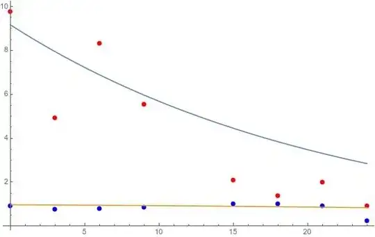
lp = ListPlot[Bdata];
p = Plot[bSol[t], {t, 0, 24}, PlotRange -> All];
Show[lp, p]
lpp = ListPlot[Sdata];
pp = Plot[sSol[t], {t, 0, 24}, PlotRange -> All];
Show[lpp, pp]

See here the fitted curves. (Blue points show $S(t)$ data and red points show $B(t)$ data.)

The fitted curve to the red points, i.e., $B(t)$, cannot capture the bump in the data around $t = 15$. I appreciate any insight or hint for how changing my ODE system slightly in order to capture this bump before falling down of the values.

EDIT

The datasets with standard deviations:

SdatawithSD = {{0, Around[9.74, 2.89]}, {3, Around[4.92, 1.65]}, {6, 
Around[8.29, 4.04]}, {9, Around[5.54, 2.45]}, {15, 
Around[2.08, 1.91]}, {18, Around[1.38, 0.962]}, {21, 
Around[1.99, 2.41]}, {24, Around[0.893, 0.359]}};
BdatawithSD = {{0, Around[0.915094, 0.1]}, {3, 
Around[0.736097, 0.091668]}, {6, Around[0.793694, 0.082575]}, {9, 
Around[0.833664, 0.070242]}, {15, Around[1, 0.002851]}, {18, 
Around[0.99578, 0.015591]}, {21, Around[0.897964, 0.04783]}, {24, 
Around[0.214499, 0.01231]}};

You may look at impulsive systems which are systems described by ODEs at almost all times but may have discontinuities at certain time instants. — KBS, Nov 26 '23 at 15:18
Please have a look first at impulsive differential equations. There are plenty of resources. Then, come back with a specific question. — KBS, Nov 26 '23 at 16:52

Cesareo · Accepted Answer · 2023-11-26T15:12:32.987

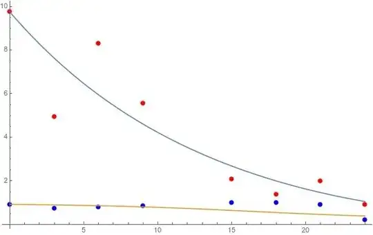
I am afraid that the bump is not natural but a consequence of the poor data set. Follows a MATHEMATICA script showing a possible best fit. The constraints are necessary to avoid singularities in the integration process.

Clear[fitness]
fitness[a00_?NumberQ, c00_?NumberQ, d00_?NumberQ, n00_?NumberQ, s0_?NumberQ, b0_?NumberQ] := Module[{ss, bb, parms, odes, ODES, solode, cinits, ssbb, lambda = 1, t},
  odes = {ss'[t] + a00/(1 + bb[t]) ss[t] == 0, bb'[t] - c00 bb[t]/(1 + ss[t]) + d00 bb[t]^2 ((1 - bb[t])/bb[t])^n00 == 0};
  cinits = {ss[0] == s0, bb[0] == b0};
  ODES = Join[odes, cinits];
  solode = Quiet@NDSolve[ODES, {ss, bb}, {t, tk[[1]], tk[[8]]}][[1]];
  Return[Sum[Norm[{y1[[k]], lambda y2[[k]]} - Evaluate[{ss[t], lambda bb[t]} /. solode /. {t -> tk[[k]]}]], {k, 1, 8}]]
  ]
tk = {0, 3, 6, 9, 15, 18, 21, 24};
y1 = {9.74, 4.92, 8.29, 5.54, 2.08, 1.38, 1.99, 0.893};
y2 = {0.915094, 0.736097, 0.793694, 0.833664, 1, 0.99578, 0.897964, 0.214499};
restrs = {0 < a00 < 0.2 && 0.2 < c00 < 0.6 && 0.1 < d00 < 0.5 && 0.3 < n00 < 1.2 + 0 0.3 && 8. < s0 < 10. && 0.01 < b0 < 0.7 + 0.3};
vars = {a00, c00, d00, n00, s0, b0};
sol = Quiet@FindMinimum[Join[{fitness[a00, c00, d00, n00, s0, b0]}, restrs], {{a00, 0.13}, {c00, 0.24}, {d00, 0.13}, {n00, 0.25}, {s0,9}, {b0, 1}}, 
   StepMonitor :> Print[{a00, c00, d00, n00, s0, b0, fitness[a00, c00, d00, n00, s0, b0]}], 
   MaxIterations -> 10, 
   WorkingPrecision -> 30]
odes = {ss'[t] + a00/(1 + bb[t]) ss[t] == 0, bb'[t] - c00 bb[t]/(1 + ss[t]) + d00 bb[t]^2 ((1 - bb[t])/bb[t])^n00 == 0} /. sol[[2]];
cinits = {ss[0] == s0, bb[0] == b0} /. sol[[2]];
ODES = Join[odes, cinits];
solode = NDSolve[ODES, {ss, bb}, {t, tk[[1]], tk[[8]]}][[1]];
gr0 = Plot[Evaluate[{ss[t], bb[t]} /. solode], {t, tk[[1]], tk[[8]]}];
gr1 = ListPlot[Transpose[{tk, y1}], PlotStyle -> Red];
gr2 = ListPlot[Transpose[{tk, y2}], PlotStyle -> Blue];
Show[gr1, gr2, gr0]

Note that lambda = 10 in necessary to make $B(t)$ data be considered as well.

NOTE

Another script, now more generic and accurate

Clear[fitness]
fitness[a00_?NumberQ, c00_?NumberQ, d00_?NumberQ, n00_?NumberQ, s0_?NumberQ, b0_?NumberQ] := 
 Module[{ss, bb, parms, odes, ODES, solode, cinits, ssbb, lambda = 10, t, tmax = tk[[8]]},
  odes = {ss'[t] + a00/(1 + bb[t]) ss[t] == 0, bb'[t] - c00 bb[t]/(1 + ss[t]) + d00 bb[t]^2 ((1 - bb[t])/bb[t])^n00 == 0,
    WhenEvent[bb[t] < 0.001, tmax = t; "StopIntegration"],
    WhenEvent[bb[t] > 0.999, tmax = t; "StopIntegration"]};
  cinits = {ss[0] == s0, bb[0] == b0};
  ODES = Join[odes, cinits];
  solode = Quiet@NDSolve[ODES, {ss, bb}, {t, tk[[1]], tk[[8]]}][[1]];
  If[tmax < tk[[8]], Return[10000/tmax]];
  Return[Sum[Norm[{y1[[k]], lambda k y2[[k]]} - Evaluate[{ss[t], lambda k  bb[t]} /. solode /. {t -> tk[[k]]}]], {k, 1, 8}]]
  ]
tk = {0, 3, 6, 9, 15, 18, 21, 24};
y1 = {9.74, 4.92, 8.29, 5.54, 2.08, 1.38, 1.99, 0.893};
y2 = {0.915094, 0.736097, 0.793694, 0.833664, 1, 0.99578, 0.897964, 0.214499};
restrs = {0 < a00 < 0.2 && 0.1 < c00 < 1 && 0.01 < d00 < 1 && 0.1 < n00 < 2 && 0.5 < s0 < 12. && 0.01 < b0 < 1};
vars = {a00, c00, d00, n00, s0, b0};
sol = Quiet@NMinimize[Join[{fitness[a00, c00, d00, n00, s0, b0]}, restrs], {a00, c00, d00, n00, s0, b0},
   Method -> "DifferentialEvolution",
   StepMonitor :> Print[{a00, c00, d00, n00, s0, b0, fitness[a00, c00, d00, n00, s0, b0]}]]
odes = {ss'[t] + a00/(1 + bb[t]) ss[t] == 0, bb'[t] - c00 bb[t]/(1 + ss[t]) + d00 bb[t]^2 ((1 - bb[t])/bb[t])^n00 == 0} /. sol[[2]];
cinits = {ss[0] == s0, bb[0] == b0} /. sol[[2]];
ODES = Join[odes, cinits];
solode = NDSolve[ODES, {ss, bb}, {t, tk[[1]], tk[[8]]}][[1]];
gr0 = Plot[Evaluate[{ss[t], bb[t]} /. solode], {t, tk[[1]], tk[[8]]}];
gr1 = ListPlot[Transpose[{tk, y1}], PlotStyle -> Red];
gr2 = ListPlot[Transpose[{tk, y2}], PlotStyle -> Blue];
Show[gr1, gr2, gr0]

The fit for S(t) and B(t) due to their range differences, (10 x 1) can be balanced with lambda. Here lambda is kind of weighting factor. — Cesareo, Nov 26 '23 at 09:05
The new script handles a feasible larger region, using an evolutive approach. The standard deviations can be included using a maximum likelihood approach. Unfortunately this is not my specialty. — Cesareo, Nov 26 '23 at 16:59
Hi again! I have asked a new question here: https://mathematica.stackexchange.com/questions/293360/how-to-include-impulses-in-differential-equations I'd be most grateful to you if you could have a look at it and see if you could help! Thanks a lot! — , Nov 28 '23 at 20:52

How to slightly modify my ODE system in order to capture bump in the data?

1 Answers1