Define the $N\times D$ matrix as $M$, then we have
$$\sigma_k(M)/\sqrt{N} \overset{\Bbb P}{\to} \sqrt{\Bbb E((x^Te_1)^2)}$$
where $\Bbb E((x^Te_1)^2)$ is a constant and can be easily estimated by Monte Carlo.
Proof:
Suppose $M$'s row vectors are $x_i\in\Bbb S^{D-1}$, fix an arbitrary $e\in\Bbb S^{D-1}$, and let
$$\mu:=\Bbb E((x^Te_1)^2),\quad v:=\Bbb V((x^Te_1)^2)$$
where $x$ follows the uniform distribution on $\Bbb S^{D-1}$. Note that $\mu(e), v(e)$ actually don't depend on $e$ so we may just write it as $\mu, v$. By Chebyshev, we have
$$\Bbb P\left(\left|\frac1N\sum_{i=1}^N(x_i^Te)^2-\mu\right| > \epsilon\right) \le \frac{v}{N\epsilon^2}$$
Therefore $\sqrt{\frac1N\sum_{i=1}^N(x_i^Te)^2}\overset{\Bbb P}{\to}\sqrt\mu$ uniformly for each $e$. This completes the proof, recalling the fact that all SVs can be defined as operator norms.
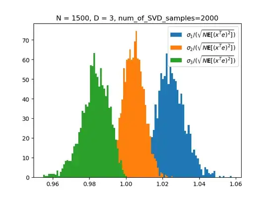
My Monte Carlo results for $D=3$:
Code:
import numpy as np
import matplotlib.pyplot as plt
def sample_spherical(npoints, ndim=3):
    vec = np.random.randn(ndim, npoints)
    vec /= np.linalg.norm(vec, axis=0)
    return vec
def get_sqrt_expectation_in_nD(ndim):
    unit_vec = np.array([[1] + [0] * (ndim - 1)])
    vec = sample_spherical(10000, ndim)
    return (((unit_vec @ vec) ** 2)[0].mean()) ** 0.5
def plot_distribution(nsamples, npoints, ndim=3):
    sv_samples = np.zeros((nsamples, ndim))
    for i in range(nsamples):
        a = sample_spherical(npoints, ndim)
        , s, _ = np.linalg.svd(a)
        sv_samples[i] = s
    expec = get_sqrt_expectation_in_nD(ndim)
    sv_samples /= expec * np.sqrt(npoints)
    for k in range(ndim):
        plt.hist(sv_samples[:, k], cumulative=False, density=True, bins=50,
                 label=r"$\sigma{%d}/(\sqrt{N{\bf{E}}[(x^Te)^2]})$" % (k + 1))
        pass
    plt.legend()
    plt.title("N = %d, D = %d, num_of_SVD_samples=%d" % (npoints, ndim, nsamples))
    return sv_samples
samples = plot_distribution(2000, 1500, 3)
