Taylor series higher-order terms

Question

I have carefully read the M.S.E. post here explaining the derivation of Taylor series, and I paid attention to the link in one of the comments, i.e., a dedicated blog post on Taylor series.

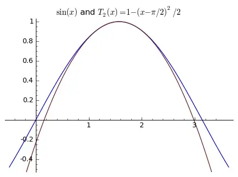
In the linked blog post, the author explains how $\sin(x)$ can be approximated with a Taylor series expansion. Specifically, an example is given for a second-order Taylor approximation (denoted $T_2(x)$) where the expansion is carried around the point $x=\frac{\pi}{2}$: here, the author explains that a curve can be defined using:

• a single point (i.e., $T_2(x=\frac{\pi}{2})=\sin(x=\frac{\pi}{2})=1$)
• the derivative at this point (i.e., we want the approximating polynomial to be $T_2'(x=\frac{\pi}{2})=\sin'(x=\frac{\pi}{2})=0$)
• The “curvature” at the same point, i.e., second derivative ($T_2''(x=\frac{\pi}{2})=\sin''(x=\frac{\pi}{2})=-1)$)

Solving for these conditions gives the following approximation:

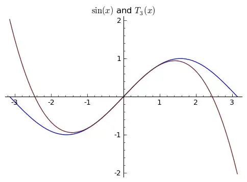
The third-order Taylor approximation, $T_3(x)$ is carried out around $x=0$ (i.e., the inflection point), by adding a condition on the third derivative at $x=0$, in addition to slope and curvature at that point, leading to:

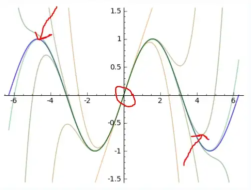
My question: I conceptually understand how the two graphs above can be generated by information at a single point (i.e., $x=\frac{\pi}{2}$ for the first one and $x=0$ for the second one). But how can higher-order derivative terms in the Taylor expansion, all taken at the same point, provide information about local minima and maxima further away from the point of the approximation?

I.e., how can higher-order derivatives taken (say) at $x=0$ see “behind the next turn”?

I try to highlight this at the graph below: I cannot get my head around how information contained at $x=0$ can give the right point for the Taylor approximation at (say) $x=\frac{3\pi}{2}$, for example.

Answer 1

This is a great question. This property, that higher derivatives at $x_0$ carry information about the behavior of the function even $x$ very far away from $x_0$ is special and not always true.

Actually, there are infinitely many infinitely differentiable functions that have the exact same derivatives at $0$ as the sine function, but which are not the sine function. (Specifically, adding scaled bump functions to sine give such functions).

The concept to look up here is called analytic functions. These are functions that are locally well-approximated by polynomials everywhere. The sine function is special, as the Taylor series at any point matches up with the function everywhere. A particular way to see why this happens is due to the (generalized) mean value theorem, or equivalently Taylor's theorem on the error. The derivatives of the sine function are bounded, and any function with bounded derivatives will also have this special property.

But other nice functions, even analytic functions, might not have this property. For example, the function $f(x) = 1/(1 + x^2)$ is analytic, but the Taylor series expanded around zero has a finite radius of convergence --- even though $f$ is well-behaved on all of $\mathbb{R}$. One explanation for this sort of behavior is that this is the restriction to $\mathbb{R}$ of the complex function $f(z) = 1/(1 + z^2)$, where $z$ is allowed to be complex. This function isn't well-behaved on all of $\mathbb{C}$, as it has a pole when $z = \pm i$. The complex analytic behavior of this function affects the real analytic behavior. This is a big topic!