How to fix discontinuities in the $\arctan$?

Question

I am working in Mathcad with the arctangent function of the following form:

$\Theta_1(t)=2\arctan(\frac{y_1(t)}{x_1(t)})$

$\Theta_2(t)=2\arctan(\frac{y_2(t)}{x_2(t)})$

where $x_1(t),y_1(t),x_2(t),y_2(t)$ - time-dependent numerators and denominators.

I want the plot of arc tangents to be displayed without "jumps" and be smooth. To do this, we need some way $±2\pi$ depending on how the numerator and denominator behave But I can't find a universal rule in any way for unwrap. I have already tried many algorithms, but none of them worked correctly everywhere.

For example: first plot shows that $\Theta_1(t)$ needs to be "down" when $sign(x_1(t))=sign(y_1(t))=1$, and where the signs are opposite, nothing needs to be taken away. But this rule will not work on the second plot. There, the first rule will cause a spike at the $0$-crossing point and "raise" the plot where it connects smoothly to neighboring areas.

New result:

Answer 1

I'm not sure how Mathcad plots work, but generally you need to evaluate the function step by step, in some order (usually increasing).

If the function value was $f(t_{i-1})$ in the previous step, then make $f(t_i)$ the value among $\Theta(t_i) +2\pi k, k \in \mathbb Z$, that is nearest to $f(t_{i-1})$.

As you said yourself, you may need to shift the outcome of your primary calculations $\Theta_{1/2}$ by $\pm2\pi$, but you cannot do so without looking at other points in time. The above algorithm gives you a continuous plot, that may in parts wander outside the $[-\pi, \pi]$ range.

Answer 2

For given functions $t\in [0,T] \mapsto (x_1(t),y_1(t))\in {\Bbb R}^2\setminus\{(0,0)\}$, I don't think that there is a general local solution to get a continuous function $\Theta_1(t)$. Take e.g. $x_1(t)=\cos(t/2), y_1(t)=\sin(t/2)$, $t\in[0,20\pi]$.

Ideally, you might want that $\Theta_1(t)=2 \arctan(\tan(t/2))=t$ should be the solution. But your software will plot a saw tooth graph with 9 discontinuities. You would have to add more and more multiples of $2\pi$ as $t$ increases. You need to have global information on the graph.

If, however, $x_1(t)$ and $y_1(t)$ comes from solving an ODE, then you may recover a continuous solution $\theta_1(t)$, simply by adding a differential equation for it to your ODE.

EDIT: Inspired by the post of @ingix, here is a suggestion using vector calculus (in a way it mimics an ODE). I use scilab (I don't know about Mathcad but assume it is close).

If $x,y$ are vectors of length $N$ describing the discretization of a smooth motion winding around the origin. Let $T=atan(x,y)$ be the arctan function taking values in $(-\pi,\pi]$. Let $DT=T(2:\$)-T(1:\$-1)$ be the vector of increments. Most of the values of $DT$ are close to zero but when the arctan jumps the value is close to $\pm 2\pi$. Calculating $R=round(DT/2 \; \pi)$ now gives values in $\{0,\pm 1\}$ and yields precisely the jumps in $T$. Using cumulative sums to recontruct the original path, $$ ST= T(1) + [0; cumsum(DT) - 2\pi \; cumsum(R)] $$ then gives you the angular path, now with discontinuities removed. (You may then multiply by 2 to get your $\Theta$).

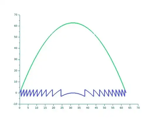
As an example I have taken some smooth curve in the plane that avoids the origin, calculated the atan along the curve ( taking values in $(-\pi,\pi]$ and giving the 'saw-tooth' blue curve). Then reconstructed the continuous angle (the green curve) from the blue curve data, using the above formulae.