Why does the Cauchy PV of $\mathsf E(1/X)$, $X\sim\mathcal N(\mu,\sigma^2)$ accurately reflect the sample mean when $|\sigma/\mu|$ is small?

Question

Suppose $X\sim\mathcal N(\mu,\sigma^2)$. The first negative moment $\mathsf E(1/X)$ does not exist; however, we can define it in the sense of the Cauchy principal value: $$ \tag{1} \mathsf E(1/X)\overset{PV}{=}\frac{\sqrt{2}}{\sigma}\,\mathcal{D}\left(\frac{\mu}{\sqrt{2}\sigma}\right), $$ where $\mathcal{D}(z)=e^{-z^{2}}\int_{0}^{z}e^{t^{2}}\,\mathrm{d}t$ is the Dawson integral. The nonexitence of the $\mathsf E(1/X)$ manifests itself in the sample mean as $$ (\overline{1/X})_n=\frac{1}{n}\sum_{k=1}^n\frac{1}{X_k} $$ never settles down to any particular value as $n$ increases ($1/X$ is in the domain of attraction of the Cauchy law and therefore does not abide by the CLT). For example, consider the running mean generated from sampling $X\sim\mathcal N(1,1)$: Because $|\sigma/\mu|$ is relatively large we regularly observe $X$ near zero and our sample mean never converges. However, in practice, this behavior is not always observed. Consider the same experiment except with sampling taken from $X\sim\mathcal N(6,1)$: We see the sample mean does settle down with increasing $n$. Moreover, the value the sample mean is approaching is the principal value moment $(1)$. In theory, this behavior is just an artifact of finite sampling in that if we continue increasing $n$ we should eventually observe values of $X$ close to zero and our sample mean will be disrupted. However, no matter how large I make $n$, I never actually observe these values in practice due to the relatively small value of $|\sigma/\mu|$.

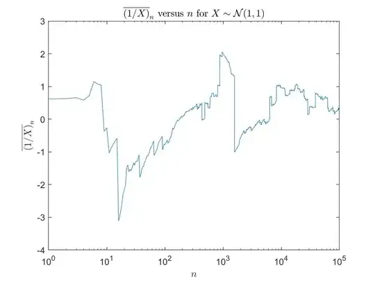
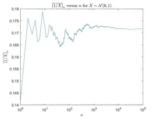
Does this make $(1)$ a useful analytical expression for the expected value $\mathsf E(1/X)$ so long as $|\sigma/\mu|$ is small? If so, what would be a coherent theoretical justification for such a statement?

For example, if $|\sigma/\mu|$ is small, we may not observe the set $\{X|\epsilon>|X|\}$ in practice and since $\mathsf E(1/X|\epsilon\leq |X|)$ exists, our sample mean is well behaved. But why should the sample mean converge to $(1)$ in this case?

Edit:

From my previous question we can further define the higher order moments $\mathsf E(1/X^m)$ for $m\in\Bbb N$ with the use of a generating function via: $$ \tag{2} \mathsf E(1/X^m):=\frac{\sqrt 2}{\sigma (m-1)!}\partial_t^{m-1}\mathcal D\left(\frac{\mu-t}{\sqrt 2 \sigma}\right)\bigg|_{t=0}. $$ As before, the sample moments $(\overline{1/X^m})_n=\frac{1}{n}\sum_{k=1}^nX_k^{-m}$ will agree with the "regularized" moments $(2)$ whenever $|\sigma/\mu|$ is small. But why?

Answer 1

If $X \sim N(\mu,\sigma)$, then $X \in (\mu - k\sigma, \mu+k\sigma)$ with probability $\Phi(k)-\Phi(-k)$, which for $k>5$ is more than $99.9999 \%$. This means that it is very unlikely, even in big samples, to observe values outside of this interval, which would also exclude values close to $0$ if $0\notin (\mu-k\sigma,\mu+k\sigma)$.

If we rather than sample from $X$ choose to sample from $X|X\in (\mu-k\sigma,\mu+k\sigma)$ (which in practice is equivalent for large $k$), then we would expect, that $$\frac1n \sum_{i=1}^n g(X_i) \rightarrow \frac{1}{\Phi(k)-\Phi(-k)} \frac{1}{\sqrt{2\pi}\sigma}\int_{\mu-k\sigma}^{\mu+k\sigma}g(x)e^{(x-\mu)^2/(2\sigma^2)} \:dx$$ for any $g \in L^1((\mu-k\sigma,\mu+k\sigma))$. So to answer your question, we must see, why $ \frac{1}{\sqrt{2\pi}\sigma}\int_{\mu-k\sigma}^{\mu+k\sigma}\frac1x e^{(x-\mu)^2/(2\sigma^2)} \:dx$ is close to the principal value of $\frac{1}{\sqrt{2\pi}\sigma}\int_{-\infty}^{\infty}\frac1x e^{(x-\mu)^2/(2\sigma^2)} \:dx$. Clearly the tails are not important, so what really matters is the principal value of $\frac{1}{\sqrt{2\pi}\sigma}\int_{-\epsilon}^{\epsilon}\frac1x e^{(x-\mu)^2/(2\sigma^2)} \:dx$ for some $\epsilon > 0$. Using the laurent series representation of $\frac1x e^{(x-\mu)^2/(2\sigma^2)}$ we can write $$\frac1x e^{(x-\mu)^2/(2\sigma^2)}=\frac{e^{-\mu^2/(2\sigma^2)}}{x} + \frac{\mu e^{-\mu^2/(2\sigma^2) }}{\sigma^2}+ O(|x|)$$ and we can thus see, that $$\int_{-\epsilon}^\epsilon \frac1x e^{(x-\mu)^2/(2\sigma^2)} \: dx \overset{PV}= 2\epsilon \frac{\mu e^{-\mu^2/(2\sigma^2) }}{\sigma^2} + O(\epsilon^2)$$ which goes to $0$ as $\epsilon$ goes to $0$.