Why are mean, median, and mode called central tendency?

Question

Is there any difference between the two terms "Central tendency" and "representative values"?
Why are mean, median, and mode called central tendency or representative values?

Answer 1

The words mean, median, and mode can apply to probability distributions or to samples. Sometimes we use the sample mean, median, and mode to help describe a sample. Sometimes we use them to esimate the mean, median, and mode of the population distribution.

Mean, median, and mode of a population. For example, consider the distribution $X \sim \mathsf{Pois}(\lambda = 1.5).$ Its mean (balance point of PDF) is 1.5. Not more than half the probability lies below its median $1$ and not more than half above.

In R:

qpois(.5, 1.5)
[1] 1
ppois(0, 1.5)
[1] 0.2231302  # P(X < 1) - 0.2231 < 0.5
1 - ppois(1, 1.5)
[1] 0.4421746  $ P(x > 1) = 1 - P(X <= 1) = 0.4422 < 0.5

Its mode is the value (if there is a unique one) that has the most probability.

k = 0:10
pdf = dpois(k, 1.5)
cbind(k, pdf)
        k          pdf
  [1,]  0 2.231302e-01
  [2,]  1 3.346952e-01  ## value with greatest probability
  [3,]  2 2.510214e-01
  [4,]  3 1.255107e-01
  [5,]  4 4.706652e-02
  [6,]  5 1.411996e-02
  [7,]  6 3.529989e-03
  [8,]  7 7.564262e-04
  [9,]  8 1.418299e-04
 [10,]  9 2.363832e-05
 [11,] 10 3.545748e-06

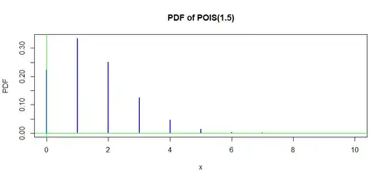
Here is a bar graph of the distribution $\mathsf{Pois}(\lambda=1.5).$

hdr = "PDF of POIS(1.5)"
plot(x, pdf, type = "h", lwd=2, col="blue",
     ylab="PDF", main=hdr)
 abline(v=0, col="green2")
 abline(h=0, col="green2")

So, for this particular Poisson distribution the median and mode happen to be the same $(1)$ and the mean is $1.5.$ In some sense each parameter calls attention to the "center" of the distribution of $X.$

Mean, median, and mode of a sample. Now, if we take a large random sample from this distribution, we can expect the sample mean, median, and mode to estimate the population mean, median and mode, respectively.

Consider the following sample of $n = 5000$ values from this distribution.

x = rpois(5000, 1.5)
summary(x)
   Min. 1st Qu.  Median    Mean 3rd Qu.    Max. 
  0.000   1.000   1.000   1.512   2.000   8.000 

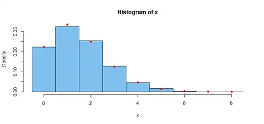
It is not difficult to find the sample mean and median. For a discrete distribution such as a Poisson distribution the tallest bar in a histogram where each bar represents a single value shows the sample mode. For a sufficiently large sample these sample measures of centrality are usually good estimates of the corresponding parameters of the population distribution.

cutp = -.5:(max(x)+.5)
hist(x, prob=T, br=cutp, col="skyblue2")
 points(k, pdf, col="red", pch=19)

The red dots show exact Poisson probabilities. as in the bar chart above.

Normal distribution. For a normal distribution, the median and mode are both the same as the population mean $\mu.$

It is easy to find the sample mean (total of observations divided by sample size) and the sample median (middle value of sorted observations; for a sample with an even number of observations, halfway between the middle two.)

In a sample from a continuous population, there may be no two observations with the same value--except possibly due to rounding. So it may not be easy to find a 'sample mode' that estimates the population mode.

Consider a sample of size 5000 from the distribution $\mathsf{Norm})\mu = 50, \sigma=7),$ for which population mean, median, and mode are all $\mu = 50.$

set.seed(1776)
y = rnorm(5000, 50, 7)
summary(y)
   Min. 1st Qu.  Median    Mean 3rd Qu.    Max. 
  23.75   45.25   49.97   49.95   54.64   75.78 

The sample mean and median are 49.95 and 49.97, respectively-- both good estimates of the $\mu = 50.$

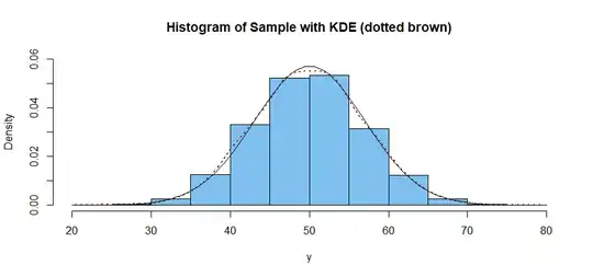
A kernel density estimator (KDE) is curve based on the sample, that seeks to imitate the density function of the population from which the sample was taken. Although the KDE has nothing to do with any one histogram of the data, it is harmless to think of a KDE as one way of "smoothing" a histogram to imitate the population density curve.

The KDE seems to reach its maximum at about 50. (The thin black curve is the density of $\mathsf{Norm}(50,7),$ which would not be known in a real application.)

hdr="Histogram of Sample with KDE (dotted brown)"
hist(y, prob=T, ylim=c(0,0.06), col="skyblue2", main=hdr)
 lines(density(y), col="brown", lwd=2, lty="dotted")
 curve(dnorm(x,50,7), add=T)

More precisely the location of the maximum of the KDE can be found to be $50,52$ as shown below. It would be reasonable to use 50.52 as the sample mode.

xx = density(y)$x;  yy = density(y)$y
mode = mean(xx[yy==max(yy)]); mode
[1] 50.51647

Answer 2

Mean, median, and mode are three different numerical descriptions of where a given data set is centred; in other words, they are different measures of its central tendency; in yet other words, they give three different average—that is, representative—values of the data set.

"Measure of central tendency" and "representative value" are both just descriptive phrases; the latter can be quite subjective: for a given data set, depending on the context, for example, its mode may be considered a more pertinent representation of its “centre” than its mean is.