7

Consider the tangent bundle $\pi:TM\to M$ for some smooth manifold. As outlined in the Wikipedia page, we can then consider the double tangent bundle via the projection $\pi_*:TTM \to TM$, with $\pi_*$ the pushforward of the canonical projection $\pi$.

In the above page, they then proceed to mention that, given $$\xi =\xi^k \frac{\partial}{\partial x^k}\Bigg|_x\in T_x M, \qquad X =X^k \frac{\partial}{\partial x^k}\Bigg|_x \in T_x M,\tag A$$ and "applying the associated coordinate system" $\xi\mapsto (x^1,...,x^n,\xi^1,...,\xi^n)$ on $TM$, the fiber on $TTM$ at $X\in T_x M$ takes the form $$(\pi_*)^{-1}(X)=\left\{ X^k\frac{\partial}{\partial x^k}\Bigg|_\xi + Y^k\frac{\partial}{\partial \xi^k}\Bigg|_\xi : \,\, \xi\in T_x M,\,\, Y^1,...,Y^n\in\mathbb R \right\}.\tag B$$ I'm struggling to understand where this expression comes from.

I think I understand that $(x^1,...,x^n,\xi^1,...,\xi^n)$ is a (local) parametrisation for $TM$, and I can see that the fiber we are interested in is $T_X TM$, that is, the set of elements of $TTM$ above $X$, but I don't understand what the expression in the last equation represents.

If I were to write a fiber $T_x M$ of the tangent bundle, this would be the set of pairs $(x,v)$ with $v$ ranging across all (equivalence classes of) smooth curves $I\to M$ passing through $x$. In local coordinates, and focusing on the "curve component" of tangent vectors, I suppose we could write this as the set $$\pi^{-1}(x)=\left\{v^k \frac{\partial}{\partial x^k}\Bigg|_x : \,\, v^k\in\mathbb R\right\}.$$ By way of analogy, I'd guess $T_X TM$ to be the set of pairs $(X,V)$ with $V$ (equivalence classes of) curves $I\to TM$ passing through $X\in T_x M$. But even switching to local coordinates, I'm not sure how to go from this description to the expression in (B).

glS
  • 7,963

2 Answers2

4

In the end, this is just a simple case of computing a tangent map and the fact that $\pi:TTM\to TM$ defines a second vector bundle structure on $TTM$ is not relevant for the problem at hand. (Partially things also get a bit complicated because you are using a notation that makes it complicated to distinguish between and object and its expression in local coordinates.)

Just start by thinking about how one constructs charts on the tangent bundle $TM$: You start with an open subset $U\subset M$ and a diffeomorphism from $U$ to an open subset $V\subset\mathbb R^n$, whose components are the local coordinates $x^i$. Denoting by $p:TM\to M$ the canonical projection, you get an induced diffeomorphism $p^{-1}(U)\to V\times\mathbb R^n$ that is used as a chart on $TM$. The first $n$ components of this are just the local coordinates $x^i$ and if you go through the construction, you see that indeed the tangent vector with coordinates $(x^1,\dots,x^n,\xi^1,\dots,\xi^n)$ exactly is $\sum_i\xi^i\tfrac{\partial}{\partial x^i}|_x$ where $x$ is the point with coordinates $x^i$. Now this shows that $(x^i,\xi^i)$ is a local coordinate system on $p^{-1}(U)\subset TM$, and hence given a point $\xi_x\in p^{-1}(U)$, any tangent vector at that point can be written as $\sum\alpha^i \tfrac{\partial}{\partial x^i}|_{\xi_x}+\sum_j\beta^j\tfrac{\partial}{\partial \xi^j}|_{\xi_x}$ for real numbers $\alpha^i$ and $\beta^j$.

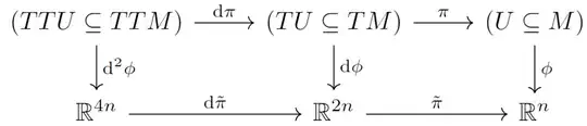
At this point, it is best to forget about vector bundle structures and all that and just notice that $\pi:TTM\to TM$ is the tangent map (i.e. the derivative) of $p:TM\to M$. Since $p$ maps $p^{-1}(U)$ to $U$, this tangent map maps $Tp^{-1}(U)$ to $TU$ and hence can be expressed in the local coordinates we have constructed. But in these local coordinates, we simply get $p(x^1,\dots,x^n,\xi^1,\dots,\xi^n)=(x^1,\dots,x^n)$. This readily shows that the tangent map sends $\tfrac{\partial}{\partial x^i}$ to $\tfrac{\partial}{\partial x^i}$ and $\tfrac{\partial}{\partial \xi^j}$ to zero. Otherwise put, $$\pi\left(\sum_i\alpha^i \frac{\partial}{\partial x^i}|_{\xi_x}+\sum_j\beta^j\frac{\partial}{\partial \xi^j}|_{\xi_x}\right)=\sum_i\alpha^i \frac{\partial}{\partial x^i}|_x$$ and this equals $\xi_x$ if and only if $\alpha^i=\xi^i$ for all $i$, which is exactly what you want to see.

Edit (to address the issue on dimensions raised in your comment): This again mainly is an issue of notation. Since you have denoted points in $M$ by $x$ and local coordinates by $x^i$, I have tried to use similar notation for tangent vectors and this gets a bit misleading. What I have actually shown above is that the tangent vector $$ T_{Y_x}p\left(\sum_i\alpha^i\tfrac{\partial}{\partial x^i}|_{Y_x}+\sum\beta^j\tfrac{\partial}{\partial \xi^j}|_{Y_x}\right)=\sum_i\alpha^i\tfrac{\partial}{\partial x^i}|_x. $$ So for fixed $Y_x$, there is an $n$-dimensional affine subspace in $T_{Y_x}TM$ that gets mapped to $X_x\in TM$. But the actual pre-image of $X_x$ in $TTM$ is the union of all these affine subspaces for all the points $Y_x$, which form an $n$-dimensional vector space. So it looks like the product of $\mathbb R^n$ with an $n$-dimensional affine subspace of $\mathbb R^{2n}$ and hence has dimension $2n$ as expected. In the expression that you wrote in the question, the $n$-missing dimensions come from the free tangent vector $\xi\in T_xM$.

Even easier, if you extend what you know about local coordinates on $TM$ to $TTM$, you see that in the notation above, we get local coordinates $(x^i,\xi^j,\alpha^k,\beta^\ell)$ on an open subset of $TTM$ and in these coordinates, we get $\pi(x^i,\xi^j,\alpha^k,\beta^\ell)=(x^i,\alpha^k)$. Hence the pre-image of $(x^1,\dots, x^n,X^1,\dots,X^n)$ has $2n$ free parameters (the $\xi^j$ and the $\beta^\ell$).

Andreas Cap
  • 22,380
  • thank you for the answer. I'm a bit confused by your notation: should the partial derivatives be defined with respect to different variables? As currently written, it looks like the sum should amount to $(\alpha^i+\beta^i)\frac{\partial}{\partial x^i}\Big|_{\xi_x}$ – glS Dec 22 '21 at 08:33
  • This is what I meant when I said your notation is confusing. These are not partial derivatives but tangent vectors in different points. Since $x^i$ can be viewed as a coordinate on $U$ and on $p^{-1}(U)$ there are such tangent vectors both in a point $x\in U$ and in a point $\xi_x\in T_xM\subset p^{-1}(U)$. And since $p$ maps between different spaces, $Tp$ changes the foot-points of tangent vectors according to $p$. – Andreas Cap Dec 22 '21 at 09:11
  • the notation is from the Wikipedia page, and yes, I agree it's confusing. Feel free to suggest a better one! I still don't understand if the two copies of $\frac{\partial}{\partial x^i}\Big|_{\xi_x}$ in the LHS of the last equation represent the same object though – glS Dec 22 '21 at 09:16
  • I am very sorry, I had a stupid copy-paste error in my answer. In two formulae I had $\frac{\partial}{\partial x^i}$ instead of $\frac{\partial}{\partial \xi^j}$. I hope that it is correct now. (And there is no double occurrence of $\frac{\partial}{\partial x^i}$ any more.) – Andreas Cap Dec 22 '21 at 13:47
  • thanks, I think I understand the gist of it now. I wanted to try and work out more precisely what exactly was going on with this notation to make sure I'm understanding it correctly, but that turned out to be way too long for a comment, so I ended up posting another answer. Feel free to let me know if I'm misunderstanding something! As far as I can tell, the gist of the matter is that the fibers contain a "horizontal part", corresponding to the $X^k$ bits in the original notation of the question, and a "vertical part" corresponding to the $Y^k$ bits – glS Dec 23 '21 at 10:02
  • however, my main point of confusion here is that both of these are supposed to be in $\mathbb R^{2n}$. In your notation, you would only seem to get $n$ dimensional fibers. Shouldn't you get $2n$ dimensions for the fibers, corresponding to the tangent component of your $\xi_x$ as well as its changes? – glS Dec 23 '21 at 10:05
  • It is a bit tricky since what you call the "vertical part" is indeed well defined (as the point-wise kernel of the tangent map of $p$) but the "horizontal part" depends on choices. I'll address the issue of dimensions in an edit to the answer. – Andreas Cap Dec 23 '21 at 19:22
0

Taking inspiration from the other answer, I'll try here to use a more rigorous/explicit notation to make sure I understand what's really going on.

Let $\pi:TM\to M$ be the canonical projection on the tangent bundle. Let $\phi:U\to\mathbb R^n$ be a chart, for some open $U\subset M$, and let $x\in U$. The double tangent bundle can be defined as the tangent bundle of $TM$ with canonical projection $\mathrm d\pi\equiv \pi_*:TTM \to TM$. Note that the local chart $(\phi,U)$ of $M$ induces the local chart $(\mathrm d\phi,TU)$ for $TM$. Finally, we also get a local chart for $TTM$ via the second differential: $(\mathrm d^2\phi,TTU)$.

Now, if we want to work in local coordinates, as done in the quote text, we have to work with the local representation of $\pi$ and $\mathrm d\pi$, that is, the maps $$ \tilde\pi\equiv \phi_* \pi\equiv \phi\circ\pi\circ \mathrm d\phi^{-1}, \qquad \tilde\pi:\mathbb R^{2n}\to\mathbb R^n, \\ \mathrm d\tilde\pi=\mathrm d\phi\circ\mathrm d\pi\circ(\mathrm d^2\phi)^{-1}, \qquad \mathrm d\tilde\pi:\mathbb R^{4n}\to\mathbb R^{2n}. $$ The relations between these maps can be summarised via the following commutative diagram:

We now observe the following:

  1. Denoting with $\{\mathbf e_i^1\}_{i=1}^n,\{\mathbf e_j^2\}_{j=1}^n\subset\mathbb R^{2n}$ bases for (subspaces of) $\mathrm d\phi(TU)$, where $\mathbf e_i^1\equiv (\mathbf e_i,\mathbf 0_n)$ and $\mathbf e_i^2\equiv(\mathbf 0_n,\mathbf e_i)$, and with $\{\mathbf e_i\}_{i=1}^n$ a basis for $\mathbb R^n$, we have $$\tilde\pi(x,v)\equiv \tilde\pi(x^i\mathbf e_i^1 + v^j\mathbf e_j^2) = x^i\mathbf e_i\equiv x.$$

  2. It follows that, denoting with $\{\mathbf e_i^3\}_{i=1}^n,\{\mathbf e_i^4\}_{i=1}^n$ linearly independent vectors to span the rest of $\mathbb R^{4n}$, we have $$ \mathrm d\tilde\pi((x,v),(\xi,\eta)) \equiv \mathrm d\tilde\pi( x^i\mathbf e_i^1 + v^j\mathbf e_j^2 + \xi^k\mathbf e_k^3 + \eta^\ell\mathbf e_\ell^4 ) \\= \tilde\pi(x^i\mathbf e_i^1 + v^j\mathbf e_j^2) + (\xi^k \partial_{\mathbf e_k^1}+\eta^\ell \partial_{\mathbf e_\ell^2})\tilde\pi(x^i\mathbf e_i^1 + v^j\mathbf e_j^2), $$ where we used the following notation for the differential of a generic smooth map $f:\mathbb R^n\to\mathbb R^m$: $$\mathrm df(\mathbf x,\mathbf v)\equiv \mathrm df(x^i\mathbf e_i + v^j \mathbf f_j) = (f(\mathbf x), v^j \partial_j f(\mathbf x)) \equiv f^i(\mathbf x)\mathbf e_i' + v^j \partial_j f^k(\mathbf x) \mathbf f_k',$$ if $\mathbf e_i',\mathbf f_i'$ are bases for the output space of $f$.

  3. Observe that $$\partial_{\mathbf e_i^1}\tilde\pi(x^i\mathbf e_i^1 + v^j\mathbf e_j^2) = \mathbf e_i, \qquad \partial_{\mathbf e_i^2}\tilde\pi(x^i\mathbf e_i^1 + v^j\mathbf e_j^2) =0, $$ and thus $$ \mathrm d\tilde\pi((x,v),(\xi,\eta)) \equiv \mathrm d\tilde\pi( x^i\mathbf e_i^1 + v^j\mathbf e_j^2 + \xi^k\mathbf e_k^3 + \eta^\ell\mathbf e_\ell^4 ) = x^i\mathbf e_i^1 + \xi^j \mathbf e_j^2 \equiv (x,\xi). \tag X$$ To match this with some geometric intuition, remember that $x^i$ parametrise a point in $U\subseteq M$, $v^i$ parametrise a tangent vector to this point, $\xi^i$ parametrise another tangent vector to the point, corresponding to the "horizontal component" of the path along $U$ we are considering, and finally $\eta^i$ parametrise tangent vectors/changes to the former tangent vectors. In particular, $\mathbf e_i^1$ and $\mathbf e_i^3$ correspond to "horizontal" directions, whereas $\mathbf e_i^2$ and $\mathbf e_i^4$ correspond to "vertical" ones.

  4. Having laid all of this groundwork, we get back to the question at hand: what do the fibers look like (in local coordinates)? In our notation, the answer is pretty straightforward: $$\mathrm d\tilde\pi^{-1}(x^i\mathbf e_i^1 + \xi^j \mathbf e_j^2) =\left\{ x^i\mathbf e_i^1 + v^j\mathbf e_j^2 + \xi^k\mathbf e_k^3 + \eta^\ell\mathbf e_\ell^4 : \,\, v^i,\eta^i\in\mathbb R \right\} \\\text{or, equivalently}\\ \mathrm d\tilde\pi^{-1}(x,\xi) = \{((x,v),(\xi,\eta)) : \,\, v,\eta\in\mathbb R^n\} \tag Y. $$

Equations (X) and (Y) are the main achievements of the above discussion. With this in mind, let me observe a few additional things to relate this expression with the notation given in the Wikipedia page, taking ideas from @peek-a-boo from the discussion in the comments:

  1. In "partial derivatives notation", we would write $\mathbf e_i^2=\frac{\partial}{\partial x^i}\Big|_x$ and $\mathbf e_i^3=\frac{\partial}{\partial x}\Big|_{x,v}$, and $\mathbf e_i^4=\frac{\partial}{\partial v^i}\Big|_{x,v}$. In this notation, the fibers we are looking look like $$\mathrm d\tilde\pi^{-1}(x,\xi) = \left\{ v^i \frac{\partial}{\partial x^i}\Bigg|_{x} + \eta^i \frac{\partial}{\partial v^i}\Bigg|_{x,v} + \xi^i \frac{\partial}{\partial x^i}\Bigg|_{x} : \,\, v^i,\eta^i\in\mathbb R \right\},$$ where it is however worth stressing that there are two copies of $\frac{\partial}{\partial x^i}$, which refer to orthogonal subspaces, although in this notation they look the same because they both represent displacements of the variable $x$. However, in this context we are effectively considering two independent ways to displace $x$, and thus we want to keep these separate in this expression.

  2. The above can equivalently be written a bit less explicitly by just prescribing $v$ to vary in the fiber $T_x M$, thus writing $$\mathrm d\tilde\pi^{-1}(x,\xi) = \left\{ \eta^i \frac{\partial}{\partial v^i}\Bigg|_{x,v} + \xi^i \frac{\partial}{\partial x^i}\Bigg|_{x} : \,\, v\in T_x M, \eta^i\in\mathbb R \right\}.$$ This expression also has the advantage of not featuring two "equal but different" copies of $\frac{\partial}{\partial x^i}$, and this is the notation used in the Wikipedia page.

glS
  • 7,963
  • haven't fully read this, but you may like to read the following answer of mine. In my notation there, given the chart on the second tangent bundle $T^2\alpha:T^2U\to (\alpha[U]\times E)\times (E\times E)$, the $\alpha[U]$ locally keeps track of the base point in $M$, the first $E$ is the fiber of $TM$ over $M$. The last two factors $(E\times E)$ are the fibers of $\pi_{TM}:T^2M\to TM$, and finally what you're interested in: the first $E$ and the last $E$ together are the fibers for $T\pi_M:T^2M\to TM$. – peek-a-boo Dec 23 '21 at 10:16
  • In other words, $(\alpha[U]\times E)\times (E\times E)\to \alpha[U]\times E$, $((x,v),(\xi,\eta))\mapsto (x,v)$ is the local form of the projection for the primary vector bundle structure $\pi_{TM}:T^2M\to TM$. For the secondary structure, i.e with respect to $T\pi_M$, it is given by $((x,v),(\xi,\eta))\mapsto (x,\xi)$. Hence, it is the set of $(v,\eta)$ which are part of the fibers (like I said above, the first and last factors of $E$); explicitly ${x}\times E\times {\xi}\times E$ is the local form of the fiber over $(x,\xi)$. – peek-a-boo Dec 23 '21 at 10:19
  • @peek-a-boo thanks for the comment, that is quite useful. I slightly edited the post to align a bit more with the notation you are using here. There is one point of confusion though: I'd say the gist of this answer is Eq. (X). Afaict, I'm considering the bundle structure $TTM\to TM$ via $\mathrm d\pi$. Is this what you call the "secondary structure"? Because I get as output the horizontal/first components of both sectors, that is, your $((x,v),(\xi,\eta))\mapsto(x,\xi)$, with $\xi$ representing changes in $x$. – glS Dec 23 '21 at 10:42
  • But I realise now this is not the same "natural canonical projection" I get considering the tangent bundle of a generic manifold, as in that case I should have $(x,v)\mapsto x$, which would translate here to $((x,v),(\xi,\eta))\mapsto (x,v)$. So, should I conclude that $\mathrm d\pi$, the pushforward of the canonical projection, is not the "most natural" canonical projection for the bundle $TTM\to TM$? Or in other words, $\mathrm d\pi$ is not the canonical projection on the tangent bundle of $TM$, where $TM$ is here thought of as a generic manifold? – glS Dec 23 '21 at 10:42
  • $T^2M$ doesn't have a "canonical" vector bundle structure. and here is why bundles are more than just sets/smooth manifolds. The projection plays a huge role. As you've observed, there are two ways to make $T^2M$ into a vector bundle over $TM$. First is to think of $N=TM$ as a generic manifold and then look at $\pi_N:TN\to N$, i.e $\pi_{TM}:T^2M\to TM$. Second is let $\pi_M:TM\to M$ be the usual tangent bundle, then take tangent mapping $T\pi_M:T^2M\to TM$ (you call this $d\pi$). You've correctly observed that these are different; this is just one of those things we live with :) – peek-a-boo Dec 23 '21 at 10:57
  • more generally if $(E,\rho,M)$ is a vector bundle, then there are two vector bundle structures for $TE$. The first is to think of $E$ as a smooth manifold, and look at $\pi_E:TE\to E$. The second is to look at $T\rho:TE\to TM$. Perhaps this slight generality may clarify the situation further (though based on your answer and comments it seems like you're already understanding the difference). – peek-a-boo Dec 23 '21 at 11:10
  • @peek-a-boo thanks, I think I'm getting it now. Though this makes me even more confused about the notation used in the Wikipedia page. They are using the pushforward as projection, so the fibers should be sets of the form, in the notation here, ${((x,v),(\xi,\eta)): v,\eta\in\mathbb R^n}$. I'm not sure how to match that with the expression they give. Their $\frac{\partial}{\partial \xi}$ makes sense, as it should correspond to our $\eta$ dof. But then they should have another sets of free parameters attached to their $\frac{\partial}{\partial x}$, which is our $v$, no? – glS Dec 23 '21 at 11:24
  • 1
    Let me modify my notation slightly to match Wikipedia. The projection we're interested in is $((x,\xi),(v,\eta))\mapsto (x,v)$. As you've agreed above, for this vector bundle structure, the fiber is ${x}\times \Bbb{R}^n\times{v}\times \Bbb{R}^n$. So, in the partial derivative notation, this set is $\left{v^i\frac{\partial}{\partial x^i}\bigg|{\xi}+\eta^i\frac{\partial}{\partial \xi^i}\bigg|{\xi},:, \xi\in T_xM, \eta^1,\dots, \eta^n\in\Bbb{R}\right}$. – peek-a-boo Dec 23 '21 at 11:43
  • 1
    The fact that we're letting $\xi\in T_xM$ be arbitrary corresponds to our first factor of $\Bbb{R}^n$ in the local form of the fiber ${x}\times \Bbb{R}^n\times {v}\times\Bbb{R}^n$. The fact that we're letting $\eta^i$ be arbitrary corresponds to our second factor of $\Bbb{R}^n$. Remember that $\frac{\partial}{\partial (\text{stuff})^i}$ only tells us directions. There's two ways to vary things. First is to multiply by appropriate coefficients (the $\eta$); the second is to plug in a different point of evaluation (the $\xi$). – peek-a-boo Dec 23 '21 at 11:44
  • 1
    Similarly, for the mapping $((x,\xi),(v,\eta))\mapsto (x,\xi)$, the fiber is ${(x,\xi)}\times \Bbb{R}^n\times\Bbb{R}^n$. Here the partial derivative notation looks like: for fixed $x\in M$ and $\xi\in T_xM$, $\left{v^i\frac{\partial}{\partial x^i}\bigg|{\xi}+\eta^i\frac{\partial}{\partial \xi^i}\bigg|{\xi},:, v^1,\dots, v^n,\eta^1,\dots, \eta^n\in\Bbb{R}\right}$. – peek-a-boo Dec 23 '21 at 11:51
  • @peek-a-boo ah, that completely clarifies it, thanks a lot! I'd incorporate parts of this discussion in the answer, if you don't mind – glS Dec 23 '21 at 12:24