9

Here is a partial inspiration for this question:

ODE: $$y''y+ax+by+c=0,y=k\pm\sqrt2\int\sqrt{a\int\ln(y)dx-(ax+c)\,\ln(y)-by+K}dx,\int\frac{dy}{\sqrt{K-(ax+c)\,\ln(y)+a\int\ln(y)dx-by}}=k\pm\sqrt2x$$

and

Is there an algebraic solution for the differential equation $y'= x^y$, and if not, can we prove this?

this is the same question, but has no current answer and only asks for a proof for a non-algebraic solution whereas I ask about a true solution.

I know it is not traditional to ask 2 questions, but I cannot choose which equation to solve, so I will solve very simple first order nonlinear differential equations:

$$y’=x^y\text{ and }y’=y^x$$

Here are the solutions:

$$y+c=\int y^x dx,y+c=\int x^y dx$$

There is also no way I can use the Frobenius method as the serie solution method.

Let’s try to separate the variables ignoring restrictions for now:

$$y’=x^y\implies \ln(y’)=y\ln(x)\implies \log_x(y’)=y\implies y’^\frac1y=x\mathop\implies^{\frac d{dx}}1=\frac{y’(x)^{\frac1y-1}(yy’’-y’^2\ln(y’))}{y^2} $$$$y’=y^x\implies y’^\frac1 x=y\implies \log_y(y’)=\frac{\ln(y’)}{\ln(y)} \mathop\implies^{\frac d{dx}} 1=\frac{y’’}{\ln(y)y’}-\frac{\ln(y’)y’}{\ln^2(y)y}$$

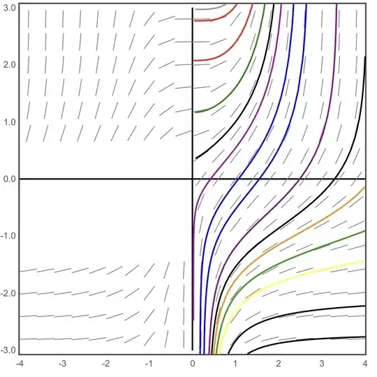
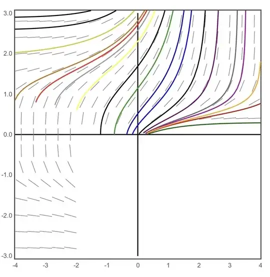
Here is the solution set family and differential curves for $y’=x^y$:

enter image description here

enter image description here

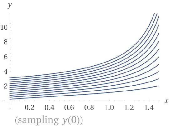
Here is the solution set family for $y’=y^x$:
enter image description here

enter image description here How do I solve for $y’=x^y$ and $y’=y^x$ for $y$ explicitly? Any series solution is appreciated. If there is a closed form, then please also write it even though it seems unlikely.

Here is some progress on $y’=x^y$ using the fact that $$x^{\sum\limits_{n\ge0} A_n}=\prod_{n\ge0} x^{A_n}:$$

$$y=\sum_{n\ge 0} a_n x^n\implies \sum_{n\ge1} a_n nx^{n-1}-\prod_{n\ge0} x^{a_n x^n} =0\implies a_1 +2 a_2 x+3 a_3x^2+…-x^{a_0}x^{a_1x}x^{a_2 x^2}\cdot …=0$$

If we were to assume that $\{a_n\}=0$, then this would not work as we have the coefficients in the exponent.

For the other differential equation, one can find the following power series using an experimental infinite Multinomial Theorem. I will also use the aforementioned Pi Product notation and factorial definition of the multinational for a representation in terms of more common functions. $n_m$ is just the mth index with the condition that the sum of all infinite number of indices is $x$. There may be a typo:

$$y’=y^x,y=\sum_{n\ge0} a_n x^n\implies\sum_{n\ge1} a_n nx^{n-1}=\left(\sum_{n\ge0}a_n x^n\right)^x\implies \sum_{n\ge1} a_n nx^{n-1}-\sum_{\sum\limits_{m\ge1} n_m=x}\frac{x!\prod\limits_{t\ge0} a_t^{n_m}x^{tn_m}}{\prod\limits_{k\ge 1}n_m!}=0$$

Here is an attempt to put $y’=x^y$ into a more manageable form using a similar method as @Cesareo’s keeping restrictions in mind. This is the corrected answer:

$$y’=x^y\implies y’’=x^{y-1}(x\ln(x)y’+y)\implies y’=x^y=\frac{xy’’}{x\ln(x)y’+y}\implies xy’’=x\ln(x)y’^2+yy’\implies\boxed{ xy’’-x\ln(x)y’^2-yy’=0}$$

which has no apparent solution so ho would I solve $$xy’’-x\ln(x)y’^2-yy’=0$$

I can think of a power series which may or may not need $2$ different indices:

$$\sum_{n=2}^\infty a_n n(n-1)x^{n-1}-x\ln(x)\sum_{n=1}^\infty a_n nx^{n-1}\sum_{n=1}^\infty a_n nx^{n-1}-\sum_{n=0}^\infty a_n x^n \sum_{n=1}^\infty a_n nx^{n-1}=0$$

We are so close to solving, so do you have any ideas? Please correct me and give me feedback!
Тyma Gaidash
  • 13,576

1 Answers1

5

Regarding the ODE $y'=y^x$.

Deriving once and substituting $y^x$ we get

$$ y'' = y'\left(\ln y + x\frac{y'}{y}\right) $$

deriving again and substituting $\ln y$ we get

$$ x y'(x)^4-y(x) y'(x)^2 \left(x y''(x)+2 y'(x)\right)+y(x)^2 \left(y'''(x) y'(x)-y''(x)^2\right)=0 $$

now calling $y_n(x) = \sum_{k=0}^n a_k x^n$ and considering $a_0,a_1,a_2$ as initial conditions we can build a series representation to $y(x)$. Follows a MATHEMATICA script which performs this task.

Clear[y]
ode = x y'[x]^4 - y[x] y'[x]^2 (2 y'[x] + x y''[x]) + y[x]^2 (-y''[x]^2 + y'[x] y'''[x])
n = 16;
xmax = 1.5;
y0 = 2.0;
delta = 0.01;
soly = NDSolve[{y'[x] == y[x]^x, y[0] == y0}, y, {x, 0, xmax}][[1]];
gr0 = Plot[Evaluate[y[x] /. soly], {x, 0, xmax}, PlotStyle -> {Thick, Blue}];
dy0 = Evaluate[y[x]^x /. soly] /. {x -> 0};
d2y0 = ((Evaluate[y[x]^x /. soly] /. {x -> delta}) - dy0)/delta/2;
cinits = {Subscript[a, 0] -> y0, Subscript[a, 1] -> dy0, Subscript[a, 2] -> d2y0};
y[x_] := Sum[Subscript[a, k] x^k, {k, 0, n}]
A = Table[Subscript[a, k] , {k, 0, n}];
coefs = Take[CoefficientList[ode, x], {1, n - 2}];
vars = Take[A, {4, n + 1}];
sol = Solve[coefs == 0, vars][[1]];
y0 = y[x] /. sol /. cinits
gr1 = Plot[y0, {x, 0, xmax}, PlotStyle -> {Thick, Dotted, Red}];
Show[gr0, gr1]

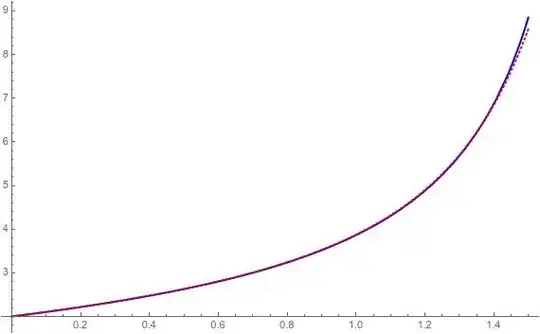
Attached a plot showing the series approximation (dotted red) in comparison with the integrated result (blue), for $y(0) = 2$.

enter image description here

NOTE

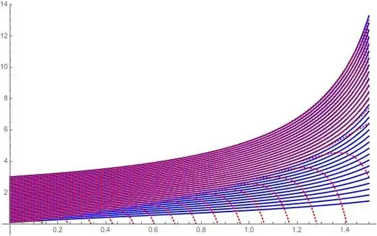
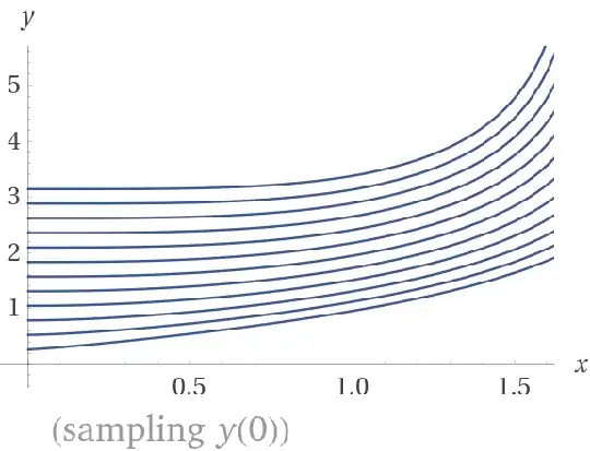
The series convergence radius depends strongly on $y(0)$ as can be observed in the following plot.

enter image description here

EDIT

Introduced the series for $n = 20$ and $y(0) = 2$

$$ y_{20}(x) = 0.0000102062 x^{20}+0.0000208849 x^{19}\\ +0.0000331216x^{18}+0.0000669035 x^{17}\\ +0.000107192 x^{16}+0.000214423 x^{15}\\ +0.00034596 x^{14}+0.000687509x^{13}\\ +0.0011134 x^{12}+0.00220569 x^{11}\\ +0.00357196 x^{10}+0.00708542 x^9\\ +0.0114163 x^8+0.0228339 x^7\\ +0.0363035 x^6+0.0742418 x^5\\ +0.11444 x^4+0.248472x^3\\ +0.350297 x^2+1. x+2. $$

EDIT-2

The first formal coefficients read

$$ \cases{ a_3\to \frac{\frac{a_1^3}{a_0}+2 a_2^2}{3 a_1}\\ a_4\to -\frac{a_1^3}{8 a_0^2}+\frac{3 a_2 a_1}{4 a_0}+\frac{a_2^3}{3 a_1^2}\\ a_5\to \frac{2 a_1^7+a_0 \left(5 a_1-12 a_2\right) a_1^5+28 a_0^2 a_2^2 a_1^3+4 a_0^3 a_2^4}{30 a_0^3 a_1^3}\\ a_6\to \frac{-30 a_1^9+5 a_0 \left(40 a_2-23 a_1\right) a_1^7+10 a_0^2\left(41 a_1-50 a_2\right) a_2 a_1^5+600 a_0^3 a_2^3 a_1^3+32 a_0^4 a_2^5}{720 a_0^4 a_1^4}\\ a_7\to \frac{36 a_1^{11}+3 a_0 \left(59 a_1-90 a_2\right) a_1^9+6 a_0^2 \left(20 a_1^2-147 a_2 a_1+130 a_2^2\right) a_1^7+12 a_0^3 \left(109 a_1-90 a_2\right) a_2^2 a_1^5+744 a_0^4 a_2^4 a_1^3+16 a_0^5a_2^6}{1260 a_0^5 a_1^5} } $$

EDIT-3

Regarding the series expansion for the ODE

$$ y'(x) = x^{y(x)} $$

after unsuccessful trials with series Frobenius inspired, we try to develop a Taylor series such as

$$ y(x) = \sum_{k=0}^n\frac{y^{(k)}(x_0)}{k!}(x-x_0)^k $$

with $y(x_0)= y_0$ the initial condition. So we have

$$ \cases{ a_0 = y_0\\ a_1 = \frac{y^{(1)}(x_0)}{1!} = x_0^{y_0}\\ a_2 = \frac{y^{(2)}(x_0)}{2!} = \frac 12 x_0^{y_0}\left(\frac{y_0}{x_0}+x_0^{y_0}\ln x_0\right)\\ a_3 = \frac{1}{3!}x_0^{y_0-2}\left(y_0(y_0-1)+2x_0^{2(y_0+1)}\ln^2 x_0-x_0^{y_0+1}(3y_0\ln x_0+2)\right)\\ \vdots } $$

This way we produce a sequence of coefficients $a_k = \Phi_k(x_0,y_0)$ and a Taylor series which converges with a convergence radius depending on the pair $\{x_0,y_0\}$. Follows a MATHEMATICA script which automatizes the procedure

Clear["Global`*"]
xmax = 1.4;
y0 = 2;
x0 = 1/2;
d[n_] := D[x^y[x], {x, n}]/n!
soly = NDSolve[{y'[x] == x^y[x], y[x0] == y0}, y, {x, x0, xmax}][[1]];
ymax = Evaluate[y[x] /. soly] /. {x -> xmax}
dy0 = x0^y0;
n = 6;
subs = {y[x] -> y0, y'[x] -> dy0, x -> x0};
d1 = x^y[x];
R = { y'[x] -> d1};
COEFS = {d1 /. subs};
For[k = 1, k <= n, k++,
 der = D[y[x], {x, k + 1}];
 d1 = D[d1, x]/(k + 1) /. R;
 AppendTo[COEFS, d1 /. subs];
 solD = Solve[der == d1, der][[1]][[1]];
 p1 = First[solD];
 p2 = Last[solD];
 If[k == 0, r1 = {p2 -> p1}, r1 = {solD}];
 AppendTo[R, r1[[1]]];
 ]
COEFS // N
fx = y0 + Sum[COEFS[[k]] (x - x0)^k, {k, 1, Length[COEFS]}] // N
gr0 = Plot[Evaluate[y[x] /. soly], {x, x0, xmax}, PlotStyle -> {Thick, Red}, PlotRange -> All];
Show[gr0, Plot[fx, {x, x0, xmax}], PlotRange -> {y0, ymax}]
Plot[Abs[fx - Evaluate[y[x] /. soly]], {x, x0, xmax}]

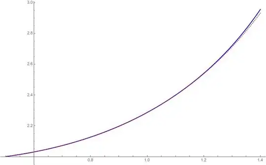
The following plot shows in red the approximation to the ODE with initial conditions $x_0 = 0.5, y_0 = 2$. Follows also the series approximation

$$ y_7(x) = 0.0124492 (x-0.5)^7+0.0653485 (x-0.5)^6+0.0943313 (x-0.5)^5+0.0166054 (x-0.5)^4+0.290859 (x-0.5)^3+0.478339 (x-0.5)^2+0.25 (x-0.5)+2. $$

enter image description here

Cesareo
  • 36,341
  • I saw the edit. This is a nice solution. I redid the other $y’=x^y$ solution, so I hope it works. Could you please list out the first 5 or so coefficients of the series solution in terms of $c_0,c_1$ etc.? I only have the Wolfram Alpha app and not Mathematica. Thanks! – Тyma Gaidash Oct 15 '21 at 21:22
  • 1
    Included the approximating series for the case study. – Cesareo Oct 15 '21 at 21:41
  • Is there an explicit for for $a_k$ like an $nth$ derivative etc? I will wait until the bounty ends in case someone else answers, but I will probably award you anyways. – Тyma Gaidash Oct 15 '21 at 21:45
  • Last thing, I plotted the first 15 terms and the differential equation in the link to desmos. Maybe it is of interest. – Тyma Gaidash Oct 15 '21 at 22:03
  • Follows the first seven coefficients. The size grows quickly making impractical to represent higher order coefficients. – Cesareo Oct 15 '21 at 22:09
  • 1
    Perfect. This will be a good solution. Thanks again! – Тyma Gaidash Oct 15 '21 at 22:09
  • This is optional, but could you please check if $$y’=x^y\implies y’’=x^{y-1}(x\ln(x)y’+y)\implies y’=x^y=\frac{yy’’}{x\ln(x)y’+y}\implies yy’’=y’ (x\ln(x)y’+y) \implies yy’’-x\ln(x)y’^2-y’y=0$$ is correct? It is at the bottom of the question.. – Тyma Gaidash Oct 18 '21 at 12:04
  • We have $y'' = x^y(\frac yx+y' \ln x)$ or $y'' = y'(\frac yx+y'\ln x)$. Take the log previously at differentiation. – Cesareo Oct 18 '21 at 12:42
  • Good job. You won the bounty. Maybe there is a way to solve $y’=x^y$? This task is optional though. – Тyma Gaidash Oct 20 '21 at 14:24
  • $y' = x^y$ resists to a series conventional approach. I hope to obtain some results... – Cesareo Oct 20 '21 at 15:39
  • 1
    I hope to see your results, I have created a possible series solution in the question to be solved. Again, this is optional to do. Thanks again. – Тyma Gaidash Oct 20 '21 at 15:40
  • 2
    @TymaGaidash Included a series approximation to $y' = x^y$. – Cesareo Oct 22 '21 at 20:42
  • I have never thought about using the Taylor Series to solve a differential equation, there should be other uses too. I will add this to my toolbox for solving. Thanks again. – Тyma Gaidash Oct 25 '21 at 18:22