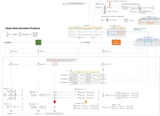
2

Gradient of $\frac{dL}{dX}$ using chain rule

With the chain rule, $\frac{dL}{dX} = \frac{dY}{dX} \cdot \frac{dL}{dY}$, and $\frac{dY}{dX} = W$ for the product Y = X•W.

Q1

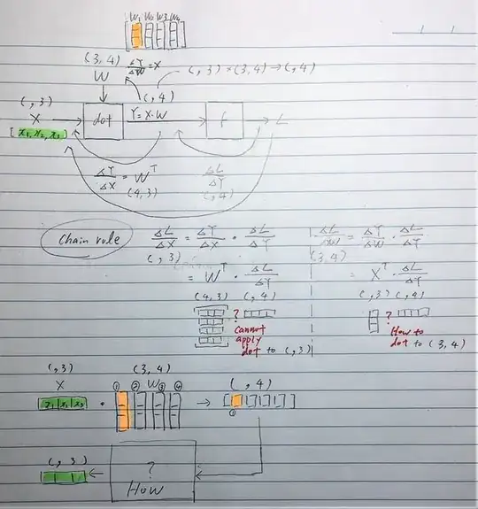
I suppose I need to make $\frac{dY}{dX}$ into a transpose $W^\intercal$ to match the shape. For instance, if X shape is (, 3) as per numpy, the last axis of shape($\frac{dY}{dX}$) needs to be 3 (so that $\frac{dY}{dX} \cdot dX^\intercal \rightarrow dY$ : (m,3) • (3,n) → (m, n)?)

However, not sure if this is correct and why, hence appreciate any explanations.

Q2

How can I apply the chain rule formula to matrix?

$\frac{dL}{dX} = W^\intercal \cdot \frac{dL}{dY}$

This cannot be calculated because of the shape mismatch where $W^\intercal$ is (4, 3) and $\frac{dL}{dY}$ is (, 4).

Likewise with $\frac{dL}{dW} = X^\intercal \cdot \frac{dL}{dY}$ because $X^\intercal$ is (,3) and $\frac{dL}{dY}$ is (, 4).

What thinking, rational or transformation can I apply to get over this?

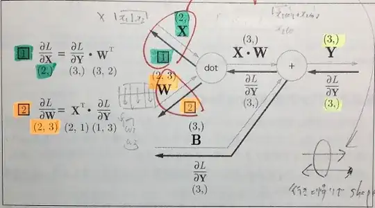
There are typos in the diagram. (,4) is (4,) etc. In my brain, 1D array of 4 element was (,4) but in NumPy, it is (4,).

enter image description here


For $\frac{dL}{dX}$

I saw the answer is swapping the positions, but no idea where it came from and why.

$\frac{dL}{dX} = \frac{dL}{dY} \cdot W^\intercal$

Instead of:

$\frac{dL}{dX} = W^\intercal \cdot \frac{dL}{dY}$

For $\frac{dL}{dW}$

The shape of $X^\intercal$ (,3) and $\frac{dL}{dY}$ (, 4) need to be transformed into (3, 1) and (1, 4) to match the shapes, but no idea where it came from and why.

enter image description here

Geometry

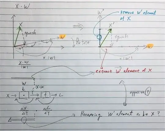
In my understanding, X•W is extracting the $\vec{\mathbf{W}}$ dimension part of X by truncating the other dimensions of X geometrically. If so, $\frac{dL}{dX}$ and $\frac{dL}{dW}$ are restoring the truncated dimensions? Not sure this is correct but if so, would it be possible to visualize it like X•W projection in the diagram?
enter image description here

mon
  • 270
  • 1
    If I am understanding correctly, you would like to find the gradient of $L = A \cdot B \equiv \operatorname{Trace}(X^T W)$ with respect to $W$, right? If yes, then my personal opinion stay away from chain rule. Better consider differentials and then compute your desired gradient. So, $dL = \operatorname{Trace}(X^T dW) \Rightarrow \frac{\partial L}{\partial W} = X$ (or it can be $\frac{\partial L}{\partial W^T} = X^T$ depending on the choice of layout) – user550103 Jan 10 '21 at 10:36
  • @user550103, thanks for the follow up. The reason chain-rule is there is because it is essential part of the neural-network (NN) back propagation. NN cascades multiple layers each contains dot, sigmoid/tanh, softmax, exp, log, etc, hence need to apply chain rule to back-track this cascade chain to get the gradients backwards through layers. – mon Jan 10 '21 at 11:18
  • 1
    If you need to calculate the weights for NN without using chain rule, then see here for instance https://math.stackexchange.com/questions/2970202/a-matrix-calculus-problem-in-backpropagation-encountered-when-studying-deep-lear – user550103 Jan 10 '21 at 12:01

1 Answers1

2

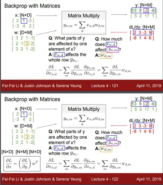
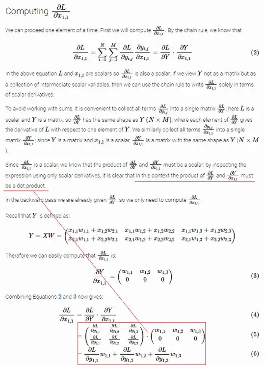
Thanks to @Reti43 for pointing to the reference. The detail math is provided by the cs231 Justin Jonson (now in Michigan University) as http://cs231n.stanford.edu/handouts/linear-backprop.pdf which is also available as Backpropagation for a Linear Layer.

cs231n lecture 4 explains the idea.

enter image description here

The math calculation from step (5) to (6) seems to be a leap, because dot product would not be resulted from two 2D matrices, and numpy.dot would produce matrix multiplication as np.matmul, hence it would not be a dot product.

The answer in numpy function to use for mathematical dot product to produce scalar addressed a way.

enter image description here


Format of the Weight vector W

Need to note on the weights representation of W by Justin Johnson.

In Coursera ML course, Andrew Ng uses a row vector to capture weights of a node. When the number of features in input to a layer is n, the row vector size is n.

Justin Johnson uses a row vector to represent a layer size, the number of nodes in a layer. Hence if there are m nodes in a layer, the row vector size is m.

Hence the weight matrix for Andrew Ng is m x n meaning m rows of weight vectors, each of which are weights for n features for a specific node.

The weight matrix for Justin Johnson is n x m meaning n rows of weight vectors, each of which are weights for m nodes in a layer, per feature.

enter image description here

I suppose Justin Johnson regards layer is a function whereas Andrew Ng regards node is a function.

As I studied Andrew Ng's ML course first, I am using weight vector per node approach which results in W as m x n matrix. My confusion came from applying W = m x n to Justin Jhonson's paper.


Understanding

My understanding by reading through the Justin Johnson's paper is below.

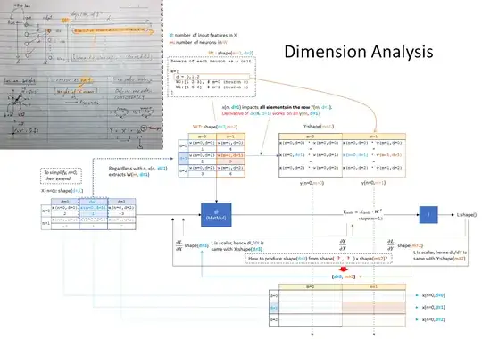
Dimension analysis

First frame the dimensions/shapes of the gradients.

enter image description here

Derive the gradient

Using the simple one input record X shape(d,), derive the dL/dX and extend it to two dimensional input X shape(n, d) resulting in dL/dY @ W. This is different from dL/dy @ W.T in the Justin Johnson's paper, because of the difference of the weight matrix W representation.

enter image description here

If something incorrect, very much appreciate any feedbacks.

mon
  • 270