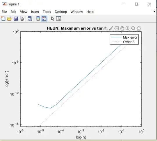
This V-shape is typical for all methods and results from the accumulation of floating point noise.
| Example |
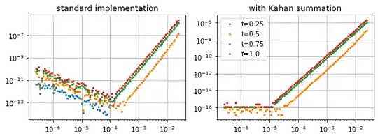 |
| Test problem $y'(t)+\sin(2y(t))=p'(t)+\sin(2p(t))$ with $p(t)=\cos(3t)$ as reference solution, integrated on $t\in[0,1]$ extracting the errors $\vert y_k-p(t_k)\vert$ for $t_k=\frac{k}4$, $k=1,2,3,4$ |
Simplified, you have error contributions proportional to $\frac{\mu_{accu}}h$ from the accumulated errors of the summation of the method steps in floating point, $\mu_{eval}$ from the ODE function evaluation, and to $h^p$ from the method itself. They balance1 at about $\mu^{1/(p+1)}$, where in a standard implementation $\mu_{accu}=\mu_{eval}=\mu=10^{-16}$ is the machine constant of 64 bit floating point numbers. This gives, for example,
for $p=2$ for the 2nd order Heun or explicit trapezoidal method (as well as the midpoint method) the minimal error at $h=\sqrt[3]\mu=10^{-5.3}$ with a value of about $h^2=10^{-10.6}$.
for a third order method like Heun's 3rd order RK method with $p=3$ an optimum at about $h=\sqrt[4]\mu=10^{-4}$ with an error level of about $h^3=10^{-12}$, which is what is represented in your graph.
for the first order Euler method the optimal $h$ at $\sqrt[2]\mu=10^{-8}$ with an error level of $h^1=10^{-8}$. You probably did not want to wait for the execution of $10^9$ steps or more, so you did not see the V-shape there but it still exists. Note that if you cut the other methods when reaching an error of $10^{-8}$, you would likewise not see the V-shape.
1: for the usual spread of trial problems, else you get contributing factors from the scales of function values and lower derivatives of the ODE function
One can try to avoid the hook for small step sizes, and continue the order slope some way down by using compensated addition in the step updates, effectively changing the number type to have a lower machine constant $\mu_{accu}\ll \mu_{eval}·h$. As one is adding many small contributions to a larger sum, some part of the updates may be lost due to rounding[2]. One can catch this defect and accumulate it until it becomes large enough to contribute to the sum in the simple floating point accuracy.
dy = 0
for k in range(N):
# For y + dy to be mostly exact it needs about double the precision of y alone
  h = t[k+1] - t[k]            # the differences in the steps might be large enough to matter
  dy += stepper(f,t[k],y[k],h) # add small to small
  y[k+1] = y[k] + dy           # next point as accurate as possible
  dy -= y[k+1] - y[k]          # remove from dy that what was actually changed in y
[2]: See https://scicomp.stackexchange.com/a/37427/6839 for some details. The (Kahan) summation trick tries to simulate a data type with doubled mantissa length.