I'm interested in how the expected cosine proximity between a vector $x\in \mathbb{R}^N$ and a perturbed version of it, $\tilde{x}=x+\varepsilon$, where $x\sim \mathcal{N}(0,\sigma I_N)$ and $\varepsilon\sim \mathcal{N}(0,\tilde{\sigma}I_N)$, scales a a function of $N$.
(EDIT: Note that I should have written $\sigma^2, \tilde{\sigma}^2$, but as the answer below uses the above notation, I will keep this as is. So, for the following, $\sigma$ denotes the variance.)
That is, what is
$$ \mathbb{E}_{x,\varepsilon}[\cos(\theta)] = \mathbb{E}_{x,\varepsilon}\left[\left\langle \frac{x}{\| x\|} \cdot \frac{\tilde{x}}{\| \tilde{x}\|} \right \rangle \right] $$
as a function of $N$?
Without loss of generality, we can assume that $\sigma = \| x \| = 1$. We cannot assume that $\tilde{\sigma} \ll \sigma$, but - if it's helpful - we could assume that $\tilde{\sigma} \leq \sigma$.
I have tried writing out the integrals, but it's a mess, and I have the feeling that there should exist a much more elegant geometric solution, which eludes me at the moment.
If there is no immediate closed-form solution to the general problem, the situation where $N\gg 1$ is the most relevant for my specific application.
EDIT: Perhaps this could be useful: Expected value of dot product between a random unit vector in $\mathbb{R}^N$ and another given unit vector
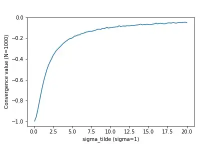
Another interesting aspect is how this expected value changes as a function of of the ratio between the two standard deviations. I have done some simulations on this:
For some ratio, the expected value always converges to some number for $N\rightarrow \infty$. In the plot below, the converged value (for $N=100$, which seemed to be more than enough) is plotted as a function of the ratio.
We clearly see that, as the size of the perturbation (captured by $\tilde{\sigma}$) increases, $x$ and $\tilde{x}$ become independent, and therefore orthogonal, which is expected.
Any insights would be appreciated!

\|instead of\vert\vertto get properly spaced double norm bars: $|$. – joriki Jan 30 '20 at 13:31