The answer to this thread states the variance for 2 Monte Carlo estimators of $\pi$.
Variance of Area and Average Estimators in Monte Carlo Estimation of Pi
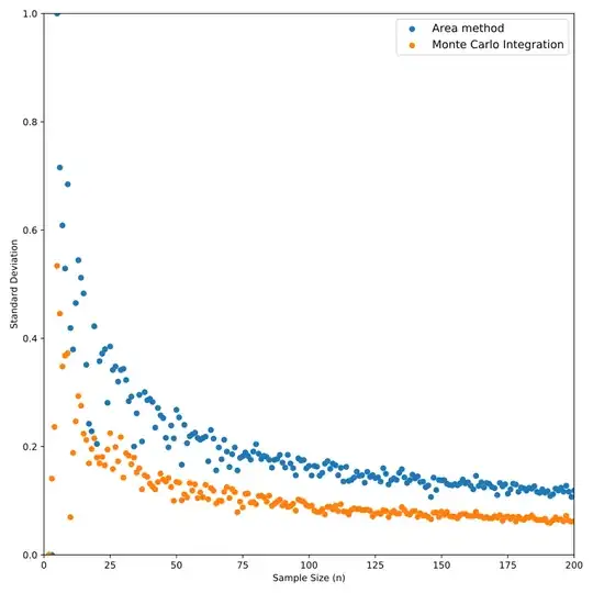
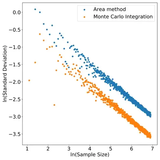
The variance for both methods is proportional to $\frac{1}{n}$, so the order of convergence must be $O(\frac{1}{\sqrt{n}})$. I am looking for a visualization of this convergence.
This is what I've done so far; it's a plot of the standard deviation with respect to the sample size. However, I'm not sure if it really captures the $O(\frac{1}{n})$ relationship. Would you have any other suggestion?
# import seaborn as sb
import numpy as np
import matplotlib.pyplot as plt
import pandas as pd
import math
# sns.set(rc={'text.usetex' : True})


plt.clf()

n = int(1e3)
pi_estimate1 = np.full(n, np.nan)
pi_estimate2 = np.full(n, np.nan)
std1 = np.full(n, np.nan)
std2 = np.full(n, np.nan)
sample_size = 1 + np.arange(n)

for i in range(n):
    np.random.seed(i)
    u1 = np.random.uniform(size = i)
    u2 = np.random.uniform(size = i)
    x = u1**2 + u2**2

    darts = np.zeros(i)
    darts[x <= 1] = 1
    in_circle_proportion = np.mean(darts)
    pi_estimate1[i] = 4 * in_circle_proportion
    std1[i] = 4*np.std(darts)/np.sqrt(i)

    sample = 4 * np.sqrt(1 - u1 ** 2)
    pi_estimate2[i] = np.mean(sample)
    std2[i] = np.std(sample)/np.sqrt(i)


plt.scatter(sample_size, std1, s = 3, label = 'Area method')
plt.scatter(sample_size, std2, s = 3, label = 'Monte Carlo Integration')
plt.xlabel("Sample Size (n)")
plt.ylabel('Standard Deviation')
plt.ylim(top = 1)
plt.ylim(bottom = 0)
plt.xlim(left = 0)
plt.xlim(right = 200)
plt.legend()
plt.show()

