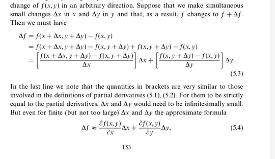
Unfortunately, this particular definition of the total differential somewhat obscures what’s really going on. IMO it’s more instructive to define it as the best linear approximation to the change in $F$ near a point. That is, the differential of $F$ at a point $\mathbf p$ is a linear map $L$ such that $\Delta F_{\mathbf p}[\mathbf h] = F(\mathbf p+\mathbf h)-F(\mathbf p) = L[\mathbf h]+o(\mathbf h).$† The function $F$ is differentiable at $\mathbf p$ if such an approximation exists. $dF$ is then a rule (function) that assigns one of these approximating linear maps to each point at which $F$ is differentiable.
In terms of a function $F:\mathbb R^2\to\mathbb R$, what this means is that near $\mathbf p$, the graph of $F$ can be approximated well by a plane—the tangent plane to $F$. To put it differently, if you zoom in close enough to a point at which $F$ is differentiable, its graph looks like a plane. The formula $dF=F_x\,dx+F_y\,dy$ is then a consequence of the above definition and the chain rule. The partial derivatives of $F$ are just the slopes of the tangent plane in the $x$ and $y$ directions, and these completely determine that plane. Note, too, that this requires a certain consistency in the way the function changes in various directions. Differentiability is a much stronger condition than simply having partial derivatives: partial derivatives only look at the slope of the graph in two directions, but to have a tangent plane the slopes have to be consistent in all directions (in fact, along all smooth curves that pass through the point).
Your concern about $F$ having huge swings in some direction is well-taken, but remember that in the differential calculus, we only examine the behavior of a function “near” a point (what your text means by “infinitesimally small”). As long as we can make the error in that linear approximation arbitrarily small by restricting our view to a small enough neighborhood of a point, all is well. You might recall from the $\epsilon-\delta$ proofs that you no doubt had to do at some point in your studies, it was sufficient to find a small enough $\delta$ for a given $\epsilon$; it didn’t matter that this might have to be very small indeed. If it turns out that no matter how much you zoom in toward a point the graph still doesn’t “flatten out” into a plane, then the function isn’t differentiable at that point. The expression $F_x\,dx+F_y\,dy$ might still be sensible at that point, but it won’t accurately represents the change in $F$ there.
By the way, if you’re near a “peak” of the graph of $F$ and $F$ is differentiable, the change in $F$ in any direction is going to be small, not large as you’re envisioning. The is the same situation as in functions of one variable: when you’re near a local maximum, the derivatives—the slopes of the graph—are near zero, and is equal to zero at the peak.
To make the development in your textbook more rigorous, you would need to carefully examine all of the sources of error in the approximation $dF$ and make sure that the total error can be made arbitrarily small. Part of this total error comes from approximating each of the difference quotients by the corresponding partial derivatives of $F$, but there’s another, more subtle source: the difference quotient ${f(x+\Delta x,y+\Delta y)\over\Delta x}$ is evaluated at $(x,y+\Delta y)$, but $F_x$ is computed at $(x,y)$.
You might also want to have a look at this question and this one, and their related questions.
† If you’re not familiar with asymptotic notation, $o(\lVert\mathbf h\rVert)$ loosely speaking means that the error in the approximation vanishes “faster” than $\mathbf h$. I.e., $f(x)=o(g(x))$ means $\lim_{x\to0}{f(x)\over g(x)}=0$. Here, this means that $\lim_{\mathbf h\to0}{\Delta F_\mathbf p[\mathbf h]-L[\mathbf h]\over\mathbf h} = 0$, which should remind you a bit of the difference quotients that you’ve seen.
