3

I am using the book Understanding Markov Chain by Nicolas Privault I start having some confusions when it comes to Continuous-Time Markov Chain.

As far as I understand, continuous-time Markov chain is quite similar to discrete-time Markov Chain, except some new formulas to find the stationary distribution by using the infinitesimal Matrix $Q$:$$\pi Q = 0$$

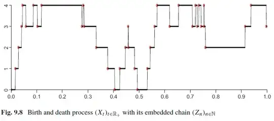
Continuous-Time Markov Chain

enter image description here

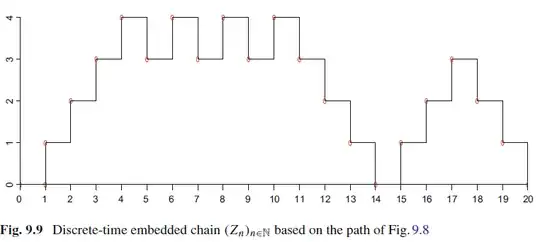
Embedded Chain (by considering only the jumps)

enter image description here

A Concrete example

Now, consider a birth and death process $X(t)$ with birth rates $\lambda_n = \lambda$ and death rates $\mu_n = n\mu$. Let $X_n$ be the embedded chain, prove that it has a stationary distribution

$$\pi_n=\frac{1}{2(n!)}(1+\frac{n}{\rho})\rho^ne^{-\rho}$$ where $\rho=\frac{\lambda}{\mu}$

My Insight

By writing out the infinitesimal Matrix and solve for $\hat{\pi} Q = 0$, we get a well known recursive relation for birth and death process.

$$\hat{\pi}_n = \frac{\lambda^{n}}{\mu^{n}n!}\hat{\pi}_0$$

Since a stationary distribution sums up to 1, we need to normalize $\hat{\pi}_n$ in order to get the real $\pi_n$. So we have:

$$\pi_n = \frac{\hat{\pi}_n}{\sum_{i=0}^{\infty}\hat{\pi}_i}$$ Since $\hat{\pi}_0$ appears on both numerator and denominator, we can cancel them out. Also notice that the denominator is actually the Talyor expansion for $e^{\rho}$. Therefore, I got

$$\pi_n=\frac{\rho^n}{e^{\rho}(n!)}$$.

Which is quite similar to the target that we want. But the problem is where are the missing terms? How do we get them back?
2 Answers2

1

First we compute the stationary distribution of $X(t)$. We have the balance equations \begin{align} \lambda\pi_0 &= \mu\pi_1\\ &\;\;\vdots\\ \lambda\pi_n &= n\mu\pi_{n+1},\quad n\geqslant 1 \end{align} from which we have the recurrence $\pi_n = \left(\frac\lambda\mu\right)^n\frac1{n!}\pi_0$. From $\sum_{n=0}^\infty \pi_n = 1$ we have $$1 = \pi_0\sum_{n=0}^\infty\left(\frac\lambda\mu\right)^n\frac1{n!}, $$ hence $\pi_0=e^-\frac\lambda\mu$ and $$\pi_n = \exp{\left(-\frac\lambda\mu\right)}\left(\frac\lambda\mu\right)^n\frac1{n!}.$$

Now consider the embedded chain $X_n$. We have transition probabilities $$ \mathbb P(X_{n+1}=j\mid X_n=i) = \begin{cases} 1,& i=0,j=1\\ \frac\lambda{\lambda+(n-1)\mu},&i>0,j=i+1\\ \frac{n\mu}{\lambda+ n\mu},& i>0,j=i-1 \end{cases} $$ Derive the balance equations and find a recurrence for $\pi_n$ in terms of $\pi_0$, then solve for $\pi_0$ to determine $\pi_n$.

Math1000
  • 38,041
0

In order to find the stationary distribution of the embedded chain one can use the discrete-time transition matrix P of the embedded chain, see for example page 251 of the book you mentioned.

The nth row of this discrete-time transition matrix P reads

$\cdots$ 0 $\frac{n}{n+\rho}$ 0 $\frac{\rho}{\rho+n}$ 0 $\cdots$

One can then check that the proposed solution solves the stationarity equation $\pi = \pi P$ for the discrete-time embedded chain.

Note that the equation $\pi Q=0$ is not satisfied here.

Andrei
  • 1
  • By $πQ=0$ is not satisfied here, do you mean that this equation can only be used to solve the continuous Chain, but not the discrete one? Also, is it always true that given a infinitesimal matrix $Q$, one can always find the transition matrix $P$? – Raven Cheuk Apr 06 '19 at 01:01
  • Yes, $\pi Q=0$ will only yield the stationary distribution of the continuous-time chain. From the infinitesimal matrix Q, one can recover the continuous-time transition semi-group P(t) of the continuous-time chain as $P(t)=\exp (tQ)$, and one can also find the discrete-time transition matrix P of the discrete-time embedded chain as in the above answer. – Andrei Apr 06 '19 at 01:23