I'm trying to solve in MatLab/Octave the advection equation, with $a > 0$ :
$$\begin{cases} u_t + au_x=0\\ u(x,0)=u^{0}(x) \end{cases}$$
with $u^{0}(x)=\begin{cases} 1.5 \quad x<0 \\0.5 \quad x>0 \end{cases}$
I have to use Lax-Wendroff's method, and then, after visualizing that the numerical solution is not 'good', use the conservative Lax-Friedrichs' method.
For a equally spaced grid both in $x$ and $t$ -axis, where the step sizes are respectively $h$ and $k$, we set $u(x_j,t_n) \approx U_j^{N}$ and use finite differences schemes in order to get, for the advection equation:
- Lax-Wendroff
$$U_j^{N+1}=U_j^N - \frac{k}{2h}a(U_{j+1}^{N}-U_{j-1}^{N}) + \frac{k^2}{2h^2}a^2(U_{j+1}^{N} - 2U_{j}^{N} + U_{j-1}^{N})$$
- Conservative Lax-Friedrichs' method:
$$U_j^{N+1}=\frac{1}{2}(U_{j+1}^{N}+U_{j-1}^{N}) - \frac{k}{2h}a(U_{j+1}^{N} - U_{j-1}^{N})$$
My doubts are basically on the computation of $U_{0}^{N}$ and $u(x_\text{final},t_n)$ with $N=1,2,\ldots$ and
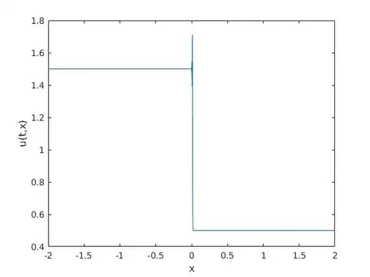
I thought to use forward and backward finite differences, using the following matlab code and getting the following figure. Please let me know if I am wrong in here
     %% Lax-Wendroff. a is a given positive number
 % the coefficients  h,k are taken in order to satisfy CFL condition
 % mt=number of time nodes in the t-axis
 % mx= number of nodes in the x-axis
 % u0 is defined as in the text.

U=zeros(mt,mx);
U(1,:)=u0;
K=(k*a)/(2*h);
KK=((k*a)^2)/(2*h^2); %re-define cfl coeff used in the iteration

for i=1:mt-1
    for j=2:mx-1
        U(i+1,j)=U(i,j) - K*(U(i,j+1)-U(i,j-1)) + KK*(U(i,j+1)-2*U(i,j)+U(i,j-1));
    end
    j=mx;
    U(i+1,1)=U(i,2) - K*(U(i,2)-U(i,1)); %first node for every time
    U(i+1,j)=(1-K^2)*U(i,j)+0.5*K*((K-1)*(2*U(i,j)-U(i,j-1))+(K+1)*U(i,j-1)); %last

    plot(x,U(i,:),'b--')
    pause(0.01)
end
end
From this image it seems that the numerical solution is not accurate enough, as expected.
\ So I use conservative Lax-Friedrichs' method. Here the problem is, as before, the computation of the values at the first and last node: I used finite differences (again) but I'm not so sure:
This is coded as follows
U=zeros(mt,mx);
U(1,:)=u0;
CFL=k/(2*h);

for i=1:mt-1
    for j=2:mx-1
         U(i+1,j)= 0.5*(U(i,j+1) + U(i,j-1)) - CFL*(U(i,j+1) - U(i,j-1));
    end
    j=mx;
    U(i+1,1)=U(i,1)-0.5*(k/h)*(U(i,2)-U(i,1)); %first x-axes node
    U(i+1,j)=U(i,j)-0.5*(k/h)*(U(i,j)-U(i,j-1)); %last x-axis node
    plot(x,U(i,:),'b--',x,u0,'r')
    legend('numerical solution','initial condition u(x,0)')
    pause(0.01)
end
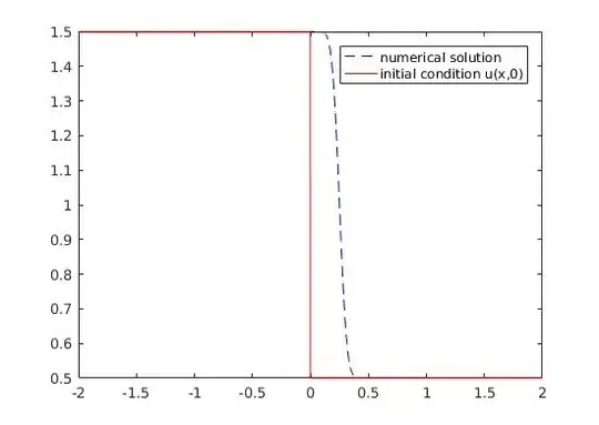
Here I got the following graphic:
Now, as you can see, the numerical solution is a little better from the previous, but I think it should not be so 'smooth' in the discontinuity.
I guess this is due to my approach in computing the values in the first and last node. How should I approximate those nodes?
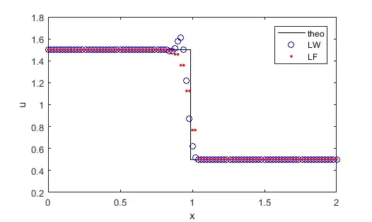
EDIT In order to see how the initial condition is trasported, using the code of @Harry49, I should write:
while (t+k)<tf
for j=2:Mx
    % Lax-Wendroff
    Utemp(1,j) = U(1,j) - 0.5*k/h*a*(U(1,j+1)-U(1,j-1)) + 0.5*(k/h*a)^2*(U(1,j+1)-2*U(1,j)+U(1,j-1));
    % Lax-Friedrichs
    Utemp(2,j) = 0.5*(U(2,j-1)+U(2,j+1)) - 0.5*k/h*a*(U(2,j+1)-U(2,j-1));
end
% Ghost cells
Utemp(:,1)    = Utemp(:,2);
Utemp(:,Mx+1) = Utemp(:,Mx);
% Update
U = Utemp;
t = t + k;
plot(x,U(1,:),'bo',x,U(2,:),'r--',[-2,a*t,a*t,2],[u0(-1),u0(-1),u0(1),u0(1)],'k-')
xlabel('x')
ylabel('u(t(i),x)')
legend('Lax Wendroff','Lax Friedrichs','Initial conditon')
axis([-2,3,0,2])
pause(0.01)

end


