I came across this post by David Bau, in which he reproduces the most widespread Mercator projection as the plot of the complex function
$$f(z)=\exp \mathrm i z.$$
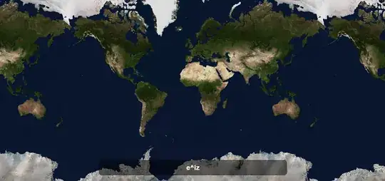
The result is familiar:
preserving the shape of the different landmasses, at the expense of enlarging the relative area of North America and Europe with respect to Equatorial and Southern Hemispherical regions.
This is equivalent to the fanning out of the top of the plot of the function on an applet provided by the same author:
Two questions:
Is the idea that if for instance, Barcelona being located at $41.3851°$ N, $2.1734°$ E, the coordinates in the $\mathbb R^2$ complex coordinates would be $41.3851 + 2.1734 \; \mathrm i,$ and after the transformation it would end up being plotted at
$f(41.3851 + 2.1734\,\mathrm i)=\exp \left(\mathrm i (41.3851 + 2.1734\,\mathrm i) \right)=-0.09734 + 0.05893\,\mathrm i$
$(-0.09734, 0.05893)$?
Is this an approximation or the exact reproduction of the actual cylindrical projection (Mercator)?
Some leg work... in R. Database is here:
> head(city)
           city   city_ascii     lat     lng    pop     country iso2 iso3 province
1 Qal eh-ye Now    Qal eh-ye 34.9830 63.1333   2997 Afghanistan   AF  AFG  Badghis
2   Chaghcharan  Chaghcharan 34.5167 65.2500  15000 Afghanistan   AF  AFG     Ghor
3   Lashkar Gah  Lashkar Gah 31.5830 64.3600 201546 Afghanistan   AF  AFG  Hilmand
4        Zaranj       Zaranj 31.1120 61.8870  49851 Afghanistan   AF  AFG   Nimroz
5    Tarin Kowt   Tarin Kowt 32.6333 65.8667  10000 Afghanistan   AF  AFG  Uruzgan
6  Zareh Sharan Zareh Sharan 32.8500 68.4167  13737 Afghanistan   AF  AFG  Paktika ...

> head(coord)
[1] 34.9830+63.1333i
    34.5167+65.2500i
    31.5830+64.3600i
    31.1120+61.8870i
    32.6333+65.8667i
    32.8500+68.4167i ...
Just plotting the raw latitude and longitude of a bunch of cities in the complex coordinates:
coord = complex(real = city$lat, imaginary = city$lng)
plot(Re(coord) ~ Im(coord), pch=20, col=rgb(0,0,0.5,.3))
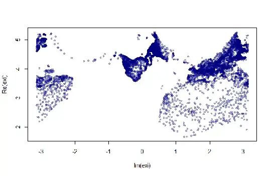
... Pretty much the Mercator map... Now transforming the dataset by simply logging the values $\log z$ renders an Azimuthal map with the South America oddly in the center:
exi = log(1i * coord)
plot(Re(exi) ~ Im(exi), pch=20, col=rgb(0,0,0.5,.3))
Perhaps the raw data in the link provided started off as logs of the latitude and longitude:


