Ultimately, the Gauss-Bonnet theorem is about the relationship between (Gaussian) curvature and "angular excess" of geodesic triangles (to be defined shortly). Once you believe in this relationship, the emergence of the Euler characteristic is just combinatorial argument involving triangulating the surface and counting the angles around all the vertices. The meat of the theorem is in angular excess.
Angular Excess and Curvature
As you know, a triangle on the unit sphere $S^2 \subset \mathbb{R}^3$ has total angle sum larger than $\pi$. Perhaps slightly less well-known is that the angular excess, that is, the quantity $\text{AE}(T) = \alpha + \beta + \gamma - \pi$, (where $\alpha,\beta,\gamma$ are the angles of our triangle $T$) is equal to the area of the triangle. This is somewhat surprising, but passes the initial smell test: small angular excess means the triangle is almost euclidean and therefore very small. Large angular excess means big angles that necessarily sweep out lots of space. Lurking behind this phenomenon is the fact that the sphere has curvature $1$, but in fact can be proven with essentially high school geometry: extend all sides of the triangle to great circles, label all angles, write down a few obvious equations, and solve the resulting system.
There's a completely analogous story in the hyperbolic plane: triangles have negative angular excess, which is again proportional to the area. This time, $\text{AE}(T) = \alpha + \beta + \gamma - \pi = -\text{Area}(T)$. I don't know of any completely elementary argument for this, but it can be done in a rather straightforward way by integration in the upper half plane model; see this answer for details.
From the constant-curvature cases, we begin to see a relationship between angular excess and area. If $k$ denotes the (constant) curvature, we might guess $$\text{AE}(T) = k\text{Area}(T).$$ This does indeed hold, but it's not clear what version of this statement should work for the non-constant case. The key idea is that, for non-constant curvature, the above equation is approximately true for very small triangles. In some heuristic sense, we have a "limit" $$\lim_{\substack{T \to \text{small}\\ p\in T}} \frac{\text{AE}(T)}{\text{Area}(T)} = K(p).$$
At this stage, it should not be at all clear that this "limit" exists, even if it were given a precise definition. Here's some fake intuition: a small piece of an arbitrary surface looks (to a second order) like a surface of constant curvature. We know that $\text{AE}(T) = k\text{Area}(T)$ holds in constant curvature, so it should hold in the limit. I call this intuition 'fake' because we have no reason to believe $\text{AE}(T)/\text{Area}(T)$ is a second order quantity. (note: $\text{AE}(T)=0$, to a first order.) A priori, it might depend on the nearby change in curvature, or worse, the shape of the triangle.
When I first saw the above heuristic limit, I really wanted to explain it away with elementary (ie non-curvature) arguments. That never worked, and I think it's because in some fundamental way, this phenomenon of angular excess-per-unit-area is curvature. In order to see this, we're going to really dig into the relationship between parallel transport, holonomy, the curvature endomorphism, and angular excess. If you're willing to take all this on faith, you can skip the next section to see the proof of Gauss-Bonnet.
Why is curvature related to angular excess?
In one sentence, it is because they are both related to parallel transportation along triangles.
Consider a triangle with vertices $A,B,C$ and angles $\alpha,\beta,\gamma$. Let $v$ be a tangent vector at $A$. We are in two dimensions, so vectors can be specified by giving their angles from specific vector; let $\theta$ be the angle between $v$ and $AC$. The plan is to see how this angle changes as we parallel translate around the triangle $A \to C \to B \to A$. (See the figure)
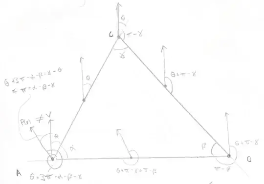
Since $AC$ is a geodesic, parallel translation of $v$ along $AC$ doesn't change the angle $\theta$. When we arrive at $C$, we will instead measure angles with respect to $BC$. This changes the angle by adding $\pi-\gamma$. Again, parallel translation along $BC$ doesn't change angle, and when we arrive at $B$ and measure angles with respect to $AB$, we pick up $\pi - \beta$. Doing this one last time, and switching measuring with respect to $AC$ again, we see that the parallel translate, $P(v)$, of $v$ along the triangle is $\theta +3\pi - \alpha - \beta - \gamma = \theta +\pi - \alpha - \beta - \gamma$ away from $AC$, and therefore $\pi - \alpha - \beta - \gamma = \text{AE}(\Delta ABC)$ away from $v$ (I just now realize there is a sign error here, which can be fixed by reversing the direction of the parallel translation sigh). Put another way, parallel translation is a rotation by angle $\text{AE}(\Delta ABC)$.
Aside: If we know that our manifold is flat (in the sense that holonomy is trivial), then we can use this argument to conclude that the angular excess of any triangle is $0$, ie angles sum to $\pi$. How delightful!
To summarize: the map $P:T_pM \to T_pM$ given by "parallel translate around the triangle $T$" is a rotation by angle $\text{AE}(T)$. We want to know show that, for small triangles, this angular excess($=$ rotation angle of $P$) is approximately $K(p)\cdot \text{Area}(T)$.
Fortunately, the curvature tensor tells us what $P$ looks like for small triangles: Let $X,Y,Z \in T_pM$. Then the parallel transport of $Z$ around the small triangle with sides $\epsilon X$ and $\epsilon Y$ is, to a second order, $P(Z) \approx Z + \frac{\epsilon^2}{2} R(X,Y)Z$. This is the standard intuitive explanation of the otherwise-scary curvature tensor. (See this question) This fact can be made suitably rigorous, but requires a somewhat lengthy calculation.
We need to find a way to extract the angle of rotation of $P$ ($=$ angular excess) from the approximation $P(Z) \approx Z + \frac{\epsilon^2}{2} R(X,Y)Z$.
This mini-section is just about rotations of $\mathbb{R}^2$ and contains no geometry. Say we have a rotation $A:\mathbb{R}^2 \to \mathbb{R}^2$ of small angle $\theta$. How can we figure out the angle $\theta$ with only infinitesimal information about where it sends vectors? Taylor expansions. (recall: $\theta$ is small) Let $v,w \in T_pM$ be an (oriented) orthonormal basis. Then $$P(v) = \cos(\theta) v + \sin(\theta) w \approx v + \theta w, \quad \text{ so } \quad \theta \approx \langle P(v), w\rangle. $$ This should make sense if you visualize the image of $v$ under a small rotation and believe $\sin(\theta) \approx \theta$.
All that remains is to piece everything together.
Let $X = \alpha_1 v + \beta_1 w$ and $Y = \alpha_2 v + \beta_2 w$ be arbitrary vectors in $T_pM$ and let $P_\epsilon$ be parallel translation along the small triangle $\Delta_\epsilon$ with legs $\epsilon X$ and $\epsilon Y$. Then $$\text{AE}(\Delta_\epsilon) \approx \text{angle of } P_\epsilon \approx \langle P(v), w \rangle \approx \langle v + \frac{\epsilon^2}{2}R(X,Y)v, w \rangle$$ Substituting in $X = \alpha_1 v + \beta_1 w$ and $Y = \alpha_2 v + \beta_2 w$, we calculate $$\langle v + \frac{\epsilon^2}{2}R(X,Y)v, w \rangle = \frac{\epsilon^2}{2}\langle R(\alpha_1 v + \beta_1 w,\alpha_2 v + \beta_2 w)v, w\rangle = \frac{\epsilon^2}{2}(\alpha_1\beta_2 - \beta_2\alpha_1)\langle R(v,w)v,w \rangle.$$ We now recognise $(\alpha_1\beta_2 - \beta_2\alpha_1) = \begin{vmatrix}\alpha_1 & \alpha_2 \\ \beta_1 &
\beta_2\end{vmatrix}$ as the area of the parallelogram spanned by $X$ and $Y$, and therefore $\frac{\epsilon^2}{2}(\alpha_1\beta_2 - \beta_2\alpha_1)$ as the area of $\Delta_\epsilon$. Putting all of this together, we have $$\text{AE}(\Delta_\epsilon) = \text{Area}(\Delta_\epsilon) \langle R(v,w)v,w \rangle = \text{Area}(\Delta_\epsilon) \cdot K(p)$$ just as required!
Woah. what just happened?
Two things:
Angular excess of a triangle is measured by parallel translating a vector along the triangle and observing how it rotates.
Parallel translating along a small triangle is measured by the curvature tensor.
The rest is calculation and commentary. Note in particular that the area of $\Delta_\epsilon$ comes from the fact that $R(X,Y)Z$ is bilinear and anti-symmetric in the first two slots, just like the $2\times 2$ determinant.
Finish off the proof of Gauss-Bonnet
The remainder of the proof of Gauss-Bonnet is purely combinatorial.
Our first observation is that angular excess is preserved under subdivisions of triangles. Specifically, let $T$ be a triangle, draw a line from a vertex to the opposite edge, and let $T_1,T_2$ be the resulting smaller triangles. Then $\text{AE}(T) = \text{AE}(T_1) + \text{AE}(T_2)$. It is easier and faster for you to do this proof by yourself than read me describe it.
Given a triangle, we can compute the angular excess in a somewhat complicated way: draw a $2\pi$ in the center of the triangle, draw a $-\pi$ by each edge, and label each angle with its value. The angular excess is then the sum of all numbers in the picture.
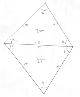
Now take a triangulation of $M$. Draw numbers in the above way. Then the "total angular excess" (ie the sum of the angular excess of all the triangles) is exactly $2\pi\chi(M)$---each vertex contributes $2\pi$ angle, each edge has two $-\pi$, and each face contributes one $2\pi$.
Subdivide the triangulation into tiny triangles. We just said this doesn't change the angular excess, so $$2\pi \chi(M) = \sum_{i = 1}^{10000} \text{AE}(T_i) \approx \sum_{i = 1}^{10000} K(p)\cdot \text{Area}(T_i) \approx \int_M KdA.$$


