If you relax your constraint to $ {x}^{T} x \leq 1 $ you can have easy solution.
I solved it for Least Squares, but it will be the same for you (Just adjust the matrices / vectors accordingly).
If you look into the solution you can infer how to deal with cases the solution has norm less than 1.
The solution below uses inversion of matrix.
But you could easily replace this step in any iterative solver of linear equation.
$$
\begin{alignat*}{3}
\text{minimize} & \quad & \frac{1}{2} \left\| A x - b \right\|_{2}^{2} \\
\text{subject to} & \quad & {x}^{T} x \leq 1
\end{alignat*}
$$
The Lagrangian is given by:
$$ L \left( x, \lambda \right) = \frac{1}{2} \left\| A x - b \right\|_{2}^{2} + \lambda \left( {x}^{T} x - 1 \right) $$
The KKT Conditions are given by:
$$
\begin{align*}
\nabla L \left( x, \lambda \right) = {A}^{T} \left( A x - b \right) + 2 \lambda x & = 0 && \text{(1) Stationary Point} \\
\lambda \left( {x}^{T} x - 1 \right) & = 0 && \text{(2) Slackness} \\
{x}^{T} x & \leq 1 && \text{(3) Primal Feasibility} \\
\lambda & \geq 0 && \text{(4) Dual Feasibility}
\end{align*}
$$
From (1) one could see that the optimal solution is given by:
$$ \hat{x} = {\left( {A}^{T} A + 2 \lambda I \right)}^{-1} {A}^{T} b $$
Which is basically the solution for Tikhonov Regularization of the Least Squares problem.
Now, from (2) if $ \lambda = 0 $ it means $ {x}^{T} x = 1 $ namely $ \left\| {\left( {A}^{T} A \right)}^{-1} {A}^{T} b \right\|_{2} = 1 $.
So one need to check the Least Squares solution first.
If $ \left\| {\left( {A}^{T} A \right)}^{-1} {A}^{T} b \right\|_{2} \leq 1 $ then $ \hat{x} = {\left( {A}^{T} A \right)}^{-1} {A}^{T} b $.
Otherwise, one need to find the optimal $ \hat{\lambda} $ such that $ \left\| {\left( {A}^{T} A + 2 \lambda I \right)}^{-1} {A}^{T} b \right\| = 1 $.
For $ \lambda \geq 0 $ the function:
$$ f \left( \lambda \right) = \left\| {\left( {A}^{T} A + 2 \lambda I \right)}^{-1} {A}^{T} b \right\| $$
Is monotonically descending and bounded below by $ 0 $.
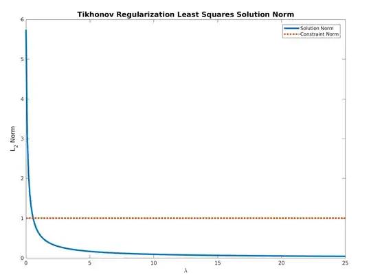
Hence, all needed is to find the optimal value by any method by starting at $ 0 $.
Basically the methods is solving iteratively Tikhonov Regularized Least Squares problem.
Remark: The above was taken from my answer to Solution for $ \arg \min_{ {x}^{T} x = 1} { x}^{T} A x - {c}^{T} x $ - Quadratic Function with Non Linear Equality Constraint.
Solve the Path of Ridge Regression Efficiently
The specific case of regularization above is basically Ridge Regression.
The objective is to calculate $ {\left( {A}^{T} A + 2 \lambda I \right)}^{-1} {A}^{T} b $ efficiently.
In order to do so, one can use the Singular Value Decomposition (SVD) of $ A = U \Sigma {V}^{T} $ which implies:
$$ A = U \Sigma {V}^{T} \implies {A}^{T} A + 2 \lambda I = V {\Sigma}^{2} {V}^{T} + 2 \lambda V {V}^{T} \implies {\left( {A}^{T} A + 2 \lambda I \right)}^{-1} {A}^{T} b = V D {U}^{T} \boldsymbol{b} $$
Where $ {D}_{ii} = \frac{ {\sigma}_{i} }{ {\sigma}_{i}^{2} + 2 \lambda } $
The above can be written as a recipe:
- Calculate the SVD of $ A $.
- Calculate $ c = {U}^{T} b $.
- Generate a single variable function $ f \left( \lambda \right) = V D \left( \lambda \right) c $.
- Use a single variable optimizer to find the $ \lambda $ which yields $ \left\| f \left( \lambda \right) \right\| = 1 $.
There are 2 cases:
- $ \left\| f \left( 0 \right) \right\| < 1 $: Then $ \lambda $ should be negative. So the optimizer search should be $ \left( -\frac{{\sigma}_{end}^2}{2}, 0 \right) $.
- $ \left\| f \left( 0 \right) \right\| > 1 $: Then $ \lambda $ should be positive. So the optimizer search should be $ \left( 0, \infty \right) $.
Remark: If $ A \in \mathbb{R}^{m \times n} $ the above will work perfectly for the overdetermined case ($ m > n $, Like in this question). For the underdetermined case it will work for the cases $ \left\| f \left( 0 \right) \right\| > 1 $. When $ m < n $ and $ \left\| f \left( 0 \right) \right\| < 1 $ then it will converge to a local minimum, but it might not be the least squares solution.
