Your goal is to stabilize the roll angle $\varphi$.
Its dynamics are described via
$$ \ddot{\varphi}I_{xx} = u $$
where $u$ is the control input (motor torque in your case).
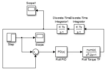
The 1$^{\text{st}}$ flaw I found is that you're using four integrators instead of two. Assuming that the measured output that is used for an output feedback control is
$$y = \int\int\ddot{\varphi}\: \text{d}t\text{d}t= \varphi,$$
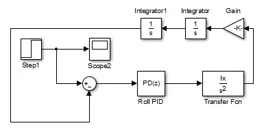
only two states are required (denoted phi and dphi in the figure). Stated as a SL model this would be

The 2$^{\text{nd}}$ problem I noted is the choice of your controller. Applying a PD controller with the transfer function
$$ K_{PD}(s) = \frac{Vs}{1+Ts} $$
renders one of your critically stable poles ($s=0$) uncontrollable due to a pole-zero cancellation in the open loop
$$ L(s) = \frac{Vs}{1+Ts} \frac{1}{s^2} = \frac{V}{s(1 + Ts)}. $$
An output-feedback controller $K$ that does the job of stabilizing the $\varphi$ can be achieved via open loop shaping. The main design goal is to retain a reasonable phase reserve of about 60°. This can be achieved by a lead/lag controller design
$$ K_{LL}(s) = V_{LL}\frac{1+T_{lead}s}{1+T_{lag}s}$$
where I chose for your nominal system ($I_{xx} = 1$) the following parameters:
$$ V_{LL} = 100, \qquad T_{lead} = \frac{1}{5}, \qquad T_{lag} = \frac{1}{50}. $$
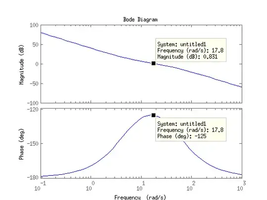
This choice yields the following Bode plot which shows a phase reserve of around 55° at a breakthrough frequency of $\omega_{c} \approx 18 \frac{\text{rad}}{\text{s}}$.
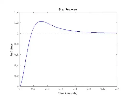
The corresponding step response gives a good idea of the performance of the controller. Note that the integrators of your model covers a vanishing control error $\lim\limits_{t\rightarrow \infty}e = 0$ for the chosen output feedback loop but I don't know if you're feeling comfortable with an overshoot of $20$%+.
In case your IMU has the capability of measuring roll velocity as well you could switch over to a state feedback controller design which has the advantage of pole placement. This means that you can freely choose thoroughly new dynamics of your roll angle behaviour (limited by input constraints and measuring noise, of course..) at the cost of losing the structural property of vanishing control error.
The Ackermann algorithm for doing so is
$$ k^T = [0, 1]S^{-1}(A,b)(p_0 + p_1A + p_2A^2), $$
where $k^T$ is the feedback vector, $S^{-1}(A,b)$ is the inverse of the controllability matrix, $A$ is your system matrix and $p_i$ are the coefficients of your desired characteristic polynomial.
Your system has the following parameters:
$$
A =
\left(
\begin{array}{cc}
0 & 1 \\
0 & 0 \\
\end{array}
\right),
\qquad
b =
\left(
\begin{array}{c}
0 \\
\frac{1}{I_{xx}} \\
\end{array}
\right),
\qquad
S(A,b) =
\left(
b, Ab
\right).
$$
I.e. your nominal system yields a feedback vector $k^T = [k_1, k_2] = [400, 40]$, given desired eigenvalues of $\lambda_1 = \lambda_2 = -20$.
It can be implemented in the following fashion:
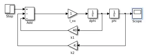
The step response needs output scaling, though:
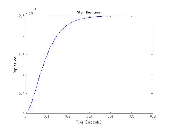
Don't forget to reassure that you don't run into any input constraints when designing the controller.