Maximum timestep for RK4

Question

I'm trying to find the maximum timestep that can be used when applying a RK4 numerical method to solve this system. I know how I would do this for single equation but have no idea how to solve it for a system of equations. Please can someone help?

$ \dfrac{d}{dt} \begin{bmatrix} y_1 \\ y_2 \end{bmatrix} = \begin{bmatrix} y_2 \\ -1.16 \ \sin(y_1) \end{bmatrix} $

---

Edit:

In terms of a model equation in the form:

$ \dfrac{dy}{dt} = \lambda y $

For the $4^{th}$ order Runge-Kutta method, the general value at a step $n+1$ is: $ y_{n+1} = y_n \ \left[ 1 + (h \lambda) + \dfrac{1}{2} (h \lambda)^2 + \dfrac{1}{6} (h \lambda)^3 + \dfrac{1}{24} (h \lambda)^4 \right]. $

So for stability:

$ \left | 1 + (h \lambda) + \dfrac{1}{2} (h \lambda)^2 + \dfrac{1}{6} (h \lambda)^3 + \dfrac{1}{24} (h \lambda)^4 \right | \leq 1. $

This is what I was saying, for a single equation, if I can rearrange my problem into the form of the model equation, I can just solve a 4th-order polynomial to determine my maximum stepsize because it must satisfy my above inequality.

But I'm confused as to how I would do it for the system of equations. The initial values of $y_1$ and $y_2$ are 2.7 and 0 respectively - at t = 0.

If we integrate your second equation only once, we get $\dfrac{dy_1}{dt} = 1.16cos(y_1) + C_1 t$. If I could work out this constant $C_1$ I would have something in the form of the model equation - as $C_1 t$ would dominate the oscillatory cosine term as $t$ gets large.

If we note that $\dfrac{dy_1}{dt} = y_2$:

$y_2 = 1.16cos(y_1) + C_1 t$

Still I'm no closer to finding $C_1$

Answer 1

As said in the comment (by user147263/Woodface), there is no real way to answer without further information. You could ask what the timestep is for an error of $10^{-6}$ or something. One also needs the integration interval.

Generally, as a fourth order method, the error is of the form $$ Ch^4+D\mu/h $$ where $\mu$ is the machine constant of the floating point type, $C,D$ are expressions in the ODE function and its derivatives. If the constants have a commensurable magnitude, the error expression has a minimum at $h=\sqrt[5]\mu\approx 10^{-3}$.

---

edit 2017: To incorporate some scale into that recommendation, chose $Lh=\sqrt[5]\mu\approx 10^{-3}$ for computations in double precision where $L$ is a Lipschitz constant, here $L=1.16$ (or its square root). Based on the shape of the stability region

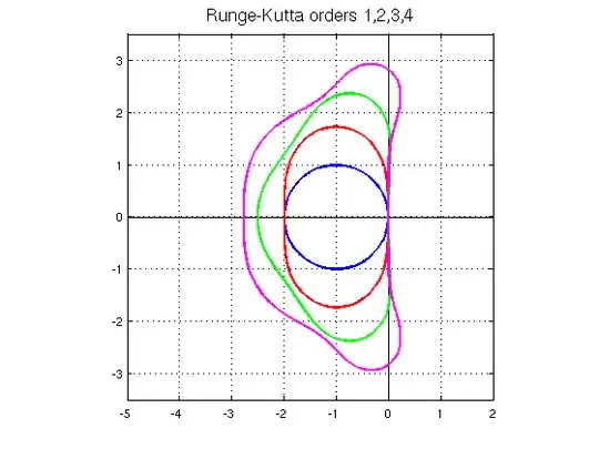
one can postulate good behavior of the RK4 method for $Lh<2.5$, as the semi-circle of that radius is contained in the stability region. As the recommended step size from the error analysis is much smaller, you should get no stability problems from error magnification.

---

(added 2/2019) Testing the various recommendations: The described test problem is the second order physical pendulum equation $$ \ddot y + 1.16\sin(y)=0, ~~ y(0)=2.7, ~~ y'(0)=0. $$ translated into first order form. The solution is about $p(t)=2.7\cos(0.6\,t)$ (closer is $2.9⋅\cos(0.5777⋅t)-0.2⋅\cos(3⋅5.777⋅t)$).

Insert this as exact solution into an MMS (method of manufactured solutions) formulation for the mapping $F[y]=\ddot y+1.16\sin(y)$, that is, $$F[y]=F[p] ~~ \text{ with } ~~ y(0)=p(0), ~~ \dot y(0)=\dot p(0) .$$

Trying out the solution and error against the exact solution for various step sizes gives the plots

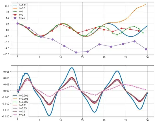
The error relates to the second plot as $e(t)=c(t)e^{0.4t}h^4$ where $c(t)$ is the function depicted.

As expected from the stability analysis, for step sizes $h=1,..,2.5$ the numerical iteration stays somewhat in the region of the exact solution for some time, while the errors grow steadily. $h=2.7$ is visibly outside the stability region for the problem.

From the error analysis one would expect the optimal step size at $h=0.001$, however as one can see in the plot, only in the range $h=0.002,..,0.1$ do the errors follow the pattern predicted by the leading error term. For $h=0.5$ the higher order error terms have too much influence, for $h=0.001$ the error pattern is disturbed by the accumulation of floating point noise.

---

(added 1/15/2021) There is a simple modification of the integration loop that makes the addition of the update approximately doubly accurate. Initialize an update vector as zero and replace

        y[i+1,:]=y[i]+(k1+2*k2+2*k3+k4)/6;

with

        update += (k1+2*k2+2*k3+k4)/6;
        y[i+1,:]=y[i]+update
        update -= y[i+1]-y[i]

This means that update accumulates the floating point errors of the step updates and shifts them to the solution if they become large enough. This, surprisingly, not only improves the result for the very small step sizes, but also for the large step sizes. Above plots, the first with unchanged parameters, the second with smaller step sizes and the exponential factor reduced to $\exp(0.05·t)$ in $e(t)=c(t)e^{0.05·t}h^4$ look now like

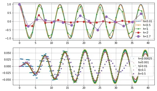
While at $h=0.00025$ one can see the granularity of the floating point type, the values still follow the error profile of the step sizes from $h=0.01$ down to $h=0.0005$. This means that the error at the smallest step size is bounded by $0.07·(0.00025)^4·e^{0.05t}= 2.734375·10^{-16}·e^{0.05t}$. Smaller errors are almost not possible in the floating point precision.

Answer 2

For the 4th order Runge Kutta scheme, the good approximated timestep to use is usually equal to or less than 0.05. Your problem is so simple that it can be easily solved in excel worksheet or it can also be easily solved with the 1st order Runge Kutta scheme.