I just finished reading the proof that the gradient is a covariant vector or a one-form, but I am having a difficult time visualizing this. I still visualize gradients as vector fields instead of the level sets associated with dual vectors. How to visualize the gradient as a one-form?
Asked
Active
Viewed 2,497 times
5
-
3The gradient is a vector field and not a one-form. The associated one-form is a different object. It can only be defined with the help of a scalar product or some other isomorphism from the tangent space to it's dual. – Thomas Jan 14 '15 at 06:06
-
According to "Spacetime and Geometry: An introduction to General Relativity" by Sean Carroll, "the simplest example of a dual vector is the gradient of a scalar function" (Carrol 20). Has Carroll made a mistake? – Jan 14 '15 at 06:08
-
1It is perhaps slightly unusual to refer to a $1$-form as a gradient. In the setting of GR, however, one generally has a background metric sitting around, and so one can equally well talk about vector fields and $1$-forms provided one is willing to identify them with the metric, so if Carroll's language is abusive, it's certainly a justifiable abuse. – Travis Willse Jan 14 '15 at 06:14
-
Okay. Thanks for the answer. – Jan 14 '15 at 06:24
-
5@Thomas: It's the other way around; the differential $df$ is always defined for real-valued function $f$ on a manifold $M$, but to define the gradient you need a map from $T^* M$ to $TM$. – Hans Lundmark Jan 14 '15 at 06:44
-
@HansLundmark Yes, you are right, of course. The message I intended to send is that you need to choose an isomorphism in order to associate the form with the vector field (and that the one-form and the vector field are not the same, of course). – Thomas Jan 14 '15 at 07:30
2 Answers
6
To clear up some confusion in the comments: when Carroll refers to the gradient of a function $f$ as a $1$-form he probably intends to refer to the exterior derivative $df$ of $f$. This is a $1$-form containing all of the information which is contained in the gradient, but which can be defined in the absence of a (pseudo-)Riemannian metric. In particular it contains precisely the data needed to differentiate $f$ with respect to any tangent vector; the result tells you how fast $f$ is changing in a particular direction at a particular point, which is what the gradient is supposed to do.
In the presence of a (pseudo-)Riemannian metric, one can identify $1$-forms and vector fields, and the vector field corresponding to $df$ along this identification is what people usually call the gradient or gradient vector field of $f$. Unlike $df$, it depends on a choice of (pseudo-)Riemannian metric. It's unusual and imprecise to refer to $df$ itself as the gradient.
Qiaochu Yuan
- 468,795
-
Thanks. You are right, because he rights the gradient as $dø$ which is the exterior derivative. – Jan 14 '15 at 06:34
-
He also defines the gradient as the set of all partial derivatives with respect to space time coordinates. – Jan 14 '15 at 06:36
2
It depends on how you like to visualize $1$-forms, but I'll assume familiarity with the "parallel planes in the tangent space" visualization:
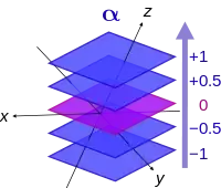
Given a function $f$ on your $n$-manifold $M$ and a point $p \in M$, we often denote the differential of $f$ at $p$ by $df_p$ (I actually prefer the less common but more "functorial" notation $T_p f$ but I'll stick to the classical notation here.) If $df_p \neq 0$, then at least near $p$, the level set $N := f^{-1}(c)$, $c := f(p)$, is a hypersurface ($(n - 1)$-manifold) through $p$, and we can think of the tangent space $T_p N$ as a hyperplane in $T_p M$.
We can identify this hyperplane readily: We can write any vector $X$ tangent to $N$ at $p$ as $X = \gamma'(0)$ for some curve $\gamma: I \to N$. Then, evaluating $df$ on $X$ gives $$df(X) = X \cdot f = \gamma'(0) \cdot f = (f \circ \gamma)'(0).$$ On the other hand, $\gamma$ is a curve in $N$, which is the set in $M$ on which $f$ takes the value $c$, so $f \circ \gamma$ is the constant function with value $c$, and $$df(X) = (f \circ \gamma)'(0) = 0.$$ Thus (counting dimensions gives that) the kernel of $df$---that is, the purple plane through the origin in the above diagram---is precisely $T_p N$. So, we can visualize the $1$-form $df_p$ as the parallel planes in $T_p M$ parallel to the hyperplane $T_p N$ tangent to the level set of $f$ through $p$.
Replacing the function $f$ with $\lambda f$ for some constant $\lambda > 1$ gives a differential $\lambda df_p$ at $p$, which has the same kernel, but more closely spaced planes, which is hence characteristic of "steeper" functions $f$.
Travis Willse
- 108,056