Improving a simple trig model

Question

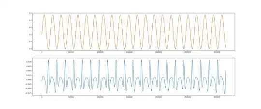
I have some data which I know is well approximated as a trig function, and I can fit it with scipy.optimize.curve_fit as follows:

from __future__import division
import numpy as np
from scipy.optimize import curve_fit 
import matplotlib.pyplot as plt
from scipy.optimize import curve_fit 



#Load the data
data = np.load('example_data.npy')

x = data[:,0]
y = data[:,1]

#Define the parametric trig function:

def trig_function(t,A,B,omega,offset):
return A*np.sin(omega*t) + B*np.cos(omega*t) + offset 

#Define fitting procedure
def fit(x,y):


    sigma = np.ones(len(t))
    sigma[[0, -1]] = 1e-1 #weight the end points

    func = trig_function #define the fitting function

    #Some guesses for initial parameter values
    dA = (y.max() + y.min()) / 2
    y_shifted = y - offset
    omega = np.pi * np.sum(y_shifted[:-1] * y_shifted[1:] < 0) / (t.max() - t.min())
    p0 = (dA,dA, omega,dA)


    #Do the fit
    popt, pcov = curve_fit(func, x,y,p0=p0,sigma=sigma)

    #return fitted data
    return func(x, *popt)

#Define plotting environment
fig = plt.figure(figsize=(24,10)) 
ax1 = plt.subplot2grid((2,1), (0,0))
ax2 = plt.subplot2grid((2,1), (1,0),sharex=ax1) 

#get fit data
y_approx = fit(x,y)

#Plot both solutions and relative error
ax1.plot(x,y)
ax1.plot(x,y_approx)
dy = (y_approx - y)/y
ax2.plot(x,dy)

This works pretty well:

However there is clearly still some feature not being accounted for by the model, especially close to the minima, as evidenced by the peaks in the relative error.

Can anyone advise how the model (i.e. the parametric trig function) could be further developed to properly account for the behaviour?

Thanks