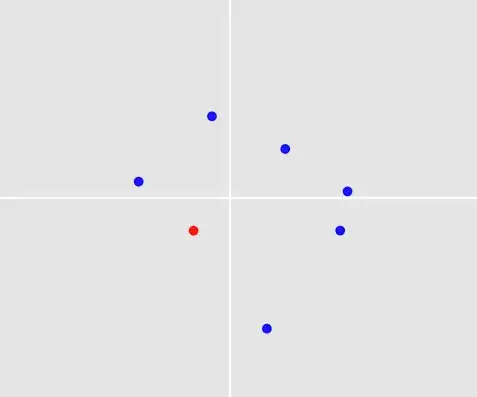
This is a fascinating problem!
Two things make it especially challenging:
- How should we compare two point sets? Classical problems in Machine Learning have a fixed number of attributes, and these attributes are not interchangeable: For example, I might have data on different persons with attributes
age and height (in centimeters). Every sample has one entry for each, and of course (age, height) = (22, 180) is not the same as (age, height) = (180, 22).
Neither is true in your problem. A point set has between 3 and 10 points, and the order in which we enter the points should not make a difference when comparing two point sets.
- How do we make a prediction? Say we have found a way to pick point sets from our training set that are similar to your point set above. We face the problem that our prediction must be one of the 7 points in your picture; but none of these points might be contained in the similar point sets.
Let me outline an algorithm that deals with both challenges. The prediction accuracy is not very good; but maybe you see a way how it can be improved. And at least it predicts something, right?
1. Simulating samples
To be able to test the algorithm, I wrote functions that generate samples and labels.
Generating samples:
Each sample contains between 3 and 10 points. The number of points is random, drawn from a uniform distribution. Each point is of the form (x_coordinate, y_coordinate). The coordinates are again random, drawn from a normal distribution.
import numpy as np
from random import randint

def create_samples(number_samples, min_points, max_points):

    def create_single_sample(min_points, max_points):
        n = randint(min_points, max_points)
        return np.array([np.random.normal(size=2) for _ in range(n)])

    return np.array([create_single_sample(min_points, max_points) for _ in range(number_samples)])
Generating labels: As a toy example, let us assume that the rule for choosing a point is: Always pick the point that is closest to (0, 0), where 'closest' should be understood in terms of the Euclidean norm.
def decision_function_minnorm(sample):
    norms = np.apply_along_axis(np.linalg.norm, axis=1, arr=sample)
    return sample[norms.argmin()]

def create_labels(samples, decision_function):
    return np.array([decision_function(sample) for sample in samples])
We can now create our train and test sets:
n_train, n_test = 1000, 100
dec_fun = decision_function_minnorm

X_train = create_samples(number_samples=n_train, min_points=3, max_points=10)
X_test = create_samples(number_samples=n_test, min_points=3, max_points=10)
y_train = create_labels(X_train, dec_fun)
y_test = create_labels(X_test, dec_fun)
2. Comparing point sets via Hausdorff distance
Let us tackle the first problem: How should we compare different point sets?
The number of points in the point sets is different.
Also remember that the order in which we write down the points should not matter: Comparing to the point set [(0,0), (1,1), (2,2)] should yield the same result as comparing to the point set [(2,2), (0,0), (1,1)].
My approach is to compare point sets via their Hausdorff distance:
def hausdorff(A, B):

    def dist_point_to_set(x, A):
        return min(np.linalg.norm(x - a) for a in A)

    def dist_set_to_set(A, B):
        return max(dist_point_set(a, B) for a in A)

    return max(dist_set_to_set(A, B), dist_set_to_set(B, A))
3. Predicting via k-nearest neighbors and averaging
We now have a notion of distance between point sets.
This makes it possible to use k-nearest neighbors classification:
Given a test point set, we find the k point sets in our training sample that have the smallest Hausdorff distance relative to the test point set, and obtain their labels.
Now comes the second problem: How do we turn these k labels into a prediction for the test point set? I took the simplest approach: average the labels and predict the point in the test point set that is closest to the average.
def predict(x, num_neighbors):
    # Find num_neighbors closest points in X_train.
    distances_to_train = np.array([hausdorff(x, x_train) for x_train in X_train])
    neighbors_idx = np.argpartition(distances_to_train, -num_neighbors)[-num_neighbors:]

    # Get labels of the neighbors and calculate the average.
    targets_neighbors = y_train[neighbors_idx]
    targets_mean = sum(targets_neighbors) / num_neighbors

    # Find point in x that is closest to targets_mean and use it as prediction.
    distances_to_mean = np.array([np.linalg.norm(p - targets_mean) for p in x])
    closest_point = x[distances_to_mean.argmin()]

    return closest_point
4. Testing
Everything is in place to test the performance of our algorithm.
num_neighbors = 70
successes = 0
for i, x in enumerate(X_test):
    print('%d/%d' % (i+1, n_test))
    prediction = predict(x, num_neighbors)
    successes += np.array_equal(prediction, y_test[i])
For the given decision function and num_neighbors = 70, we get a prediction accuracy of 84%.
This is not terribly good, and it is of course specific to our decision function, which seems fairly easy to predict.
To see this, define a different decision function:
decision_function_maxaverage(sample):
    avgs = (sample[:, 0] + sample[:, 1]) / 2
    return sample[norms.argmin()]
Using this function via dec_fun = decision_function_maxaverage brings down prediction accuracy to 45%.
This shows how important it is to think about the decision rules that generate your labels. If you have an idea why people choose certain points, this will help you find the best algorithm.
Some ways to improve this algorithm: (1) Use a different distance function instead of Hausdorff distance, (2) use something more sophisticated than k-nearest neighbors, (3) improve how the selected training labels are turned into a prediction.
