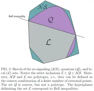
So, the first comment is that we know that the quantum body itself is not a polytope because we may find cases in which the extremal points form a continuum of points instead of just a finite set of points. In this recent paper here they have even plotted sections of this body, and you can see the boundaries. In particular, the ones I liked the most are the elliptopes. The results there also show that this body cannot be a polytope. This is rigorously proved there in full detail, and I here outline a particular argument that might be more 'easy' as the question asks for.
One can see that for the restricted case, the quantum correlations satisfy the equation $1-x^2-y^2-z^2+2xyz \geq 0$ as in the above cited paper. The procedure is the following:
Let $c=(\langle A_1B_1\rangle,\langle A_1B_2\rangle,\langle A_2B_1\rangle,\langle A_2B_2\rangle) = (1,x,y,z)$. Now, since we have dichotomic measurements we can model $\langle A_iB_j \rangle = 2p(A_i=B_j)-1$. The set $p(A_i=B_j) = \text{Tr}(P^{A_i}_0 P^{B_j}_0)$ if we have set of outcomes $\{0,1\}$. All information in the correlations is then encoded in these traces.
Let's then make $\langle A_1B_1\rangle = 1$. We may then fix $P_0^{A_1} = P_0^{B_1} = \vert 0 \rangle \langle 0 \vert$. Instead of writing the projector I can equivalently write the vectors $\vert A_2^0 \rangle, \vert B_2^0 \rangle$ for the remaining states $P_0^{A_2} = \vert A_2^0 \rangle \langle A_2^0 \vert$ and same for $P_0^{B_2}$. I want then to optimize this section of the quantum body. In general, correlations can be described if we choose the vectors,
$$\vert A_2^0 \rangle = \cos(\beta)\vert 0 \rangle + \sin(\beta)\vert 1 \rangle$$
$$\vert B_2^0 \rangle = \cos(\gamma)\vert 0 \rangle + \sin(\gamma)\cos(\alpha)e^{i\theta}\vert 1 \rangle + \sin(\gamma)\sin(\alpha)\vert 2 \rangle$$
In this description, CHSH becomes $$1 \geq c_{12}+c_{21}-c_{22} = \langle A_1B_2\rangle + \langle A_2B_1\rangle-\langle A_2B_2\rangle (A_1=B_1) \\= 2\text{Tr}(P^{A_1}_0 P^{B_2}_0)-1 + 2\text{Tr}(P^{A_2}_0 P^{B_1}_0)-1-(2\text{Tr}(P^{A_2}_0 P^{B_2}_0)-1)
\\\implies 2\text{Tr}(P^{A_1}_0 P^{B_2}_0)-1 + 2\text{Tr}(P^{A_2}_0 P^{B_1}_0)-1-(2\text{Tr}(P^{A_2}_0 P^{B_2}_0)-1) \leq 1
\\\implies 2\text{Tr}(P^{A_1}_0 P^{B_2}_0)-1 + 2\text{Tr}(P^{A_2}_0 P^{B_1}_0)-2\text{Tr}(P^{A_2}_0 P^{B_2}_0)\leq 1
\\\implies 2\text{Tr}(P^{A_1}_0 P^{B_2}_0) + 2\text{Tr}(P^{A_2}_0 P^{B_1}_0)-2\text{Tr}(P^{A_2}_0 P^{B_2}_0)\leq 2
\\\implies \text{Tr}(P^{A_1}_0 P^{B_2}_0) + \text{Tr}(P^{A_2}_0 P^{B_1}_0)-\text{Tr}(P^{A_2}_0 P^{B_2}_0)\leq \frac{1}{2}2
\\\implies \text{Tr}(P^{A_1}_0 P^{B_2}_0) + \text{Tr}(P^{A_2}_0 P^{B_1}_0) - \text{Tr}(P^{A_2}_0 P^{B_2}_0) \leq 1 \implies f \leq 1$$ but this implies that the maximum quantum set can be obtained from maximizing the CHSH term $f$ for this fact of the convex body. Meaning we may maximize the quantity:
$$f(\alpha,\beta,\gamma,\theta) = cos^2(\gamma)+\cos^2(\beta)-\cos^2(\gamma)\cos^2(\beta)+\sin^2(\gamma)\sin^2(\beta)\sin^2(\alpha)-2\sin(\gamma)\cos(\gamma)\sin(\beta)\cos(\beta)\sin(\alpha)\cos(\theta)$$
This can be done analytically (see the appendix of this paper here, published here) and the resulting equation is an equation that is not a polytope but corresponds to a continuous boundary curve, which is the same as the elliptope curve, but now for the traces instead of for the correlations (but this is a dual maximization representation for this particular case).
