The random walkers' first meeting

Question

Consider a discrete, one-dimensional, space made of $N$ squares. At the extremes of this space (so in position $1$ and $N$ respectively) two random walkers are placed, at time $t=0$ (time is discrete). At each new time $t'=t+1$ they have probability $1/3$ of staying still, moving left, or moving right. If they try to escape the space between $1$ and $N$ they simply stay still, nothing happens, so a kind of reflective barrier is in place. What is the shape of the discrete probability distribution of the walkers' first encounter? It will be a normalized vector of dimension equal to $N$ of course.

Also consider this: The walkers move at the same time, so if the walkers end up in adjacent squares they could pass over one another in the next move; this should not be possible: any compenetration is considered an encounter, and the square of encounter is randomly chosen between the two previous occupied squares.

Answer 1

By scaling everything by $1/N$, we can compute the limiting density of the first encounter location. We can get it in closed form, but only in terms of elliptic functions. Namely, the limiting density over $t \in [0, 1]$ is $$ g(t) = \frac{4K(-1)}{\pi}\sqrt{\frac{\varphi(t)^{2} - \varphi(t)^{-2}}{2i}}, $$ where $K$ is the complete elliptical function and $\varphi$ is defined by $$ \varphi(t) = \operatorname{sn}(K(-1)(1 + (i-1)t), -1), $$ where $\operatorname{sn}$ is the Jacobi elliptic sine function.

These special functions are complicated, but standard enough to be implemented in common special function libraries. So for instance, we can implement this in R easily enough:

library(elliptic)
n_grid <- 1000
t_grid <- seq(0, 1, length.out = n_grid)
z_grid <- 1 + (-1 + 1i) * t_grid
phi <- sn(K.fun(-1) * z_grid, -1)
dmu <- K.fun(-1) * 4/pi * sqrt((phi^2 - phi^(-2))/(2i))

The complete proof is involved, the ideas are as follows:

1. As per Greg Martin's observation, this problem is equivalent to finding the distribution of the first location that a random walker on an $N \times N$ grid crosses the diagonal $\{(k, k) : k\in 1, \dotsc, N\}$

2. By reflecting the sample paths along the axes, the above problem can further be translated to finding the first location that a random walker starting at $(0, 0)$ first leaves the diamond $\{(x, y) : |x| + |y| < N\}$ (this is not an exact correspondence because the reflection is not so easy, but the discrepancy disappears in the limit)

3. Taking the limit as $N \rightarrow \infty$, this becomes the problem of finding the point at which a 2-d Brownian motion leaves the diamond $V = \{(x, y) : |x| + |y| \leq 1\}$ - a classical result is that this is the harmonic measure for the unit diamond.

4. This harmonic measure $\mu$ is constructed from the Riemann map from the unit disc $D$ to the unit diamond. That is, if $f \colon D \rightarrow V$ is a conformal map with $f(0) = 0$, the density of the measure is $$ \frac{\mathrm{d}\mu(w)}{\mathrm{dw}} = \frac{1}{2\pi i}\frac{\psi'(w)}{\psi(w)}, $$ where $\psi = f^{-1}$.

5. Since $V$ is a polygon, the conformal map $f$ is a Schwarz-Christoffel map. The unit diamond has a particularly nice such map, allowing us to write its derivative explicitly as $$ f'(z) = \frac{1}{K(-1)(1 - z^4)^{1/2}}, $$ with its antiderivative being defined in terms of the elliptic integral of the first kind $F$ according to $f(z) = F(z; -1)/K(-1)$. The inverse of these functions is defined in terms of Jacobi elliptic functions, rendering $$ \psi(w) = f^{-1}(w) = \operatorname{sn}(K(-1)w, -1). $$

   But now we can write \begin{align*} \frac{\mathrm{d}\mu(w)}{\mathrm{d}w} &= \frac{1}{2\pi i}\frac{\psi'(w)}{\psi(w)} \\ &= \frac{1}{2\pi i}\frac{1}{\psi(w)f'(\psi(w))} \\ &= \frac{K(-1)}{2\pi i} \sqrt{\psi(w)^{-2} - \psi(w)^2} \end{align*}

6. We transfer back from the diamond to the unit interval by making the transformation $$ w = 1 + (i-1) t, \quad \varphi(t) = \psi(w) $$ mapping the interval to one edge of the diamond. This transformation picks up a factor of $(i-1)$, as we multiply by $4$ to account for the fact that the Brownian motion can escape through any of the four edges, so the final form of the density is \begin{align*} g(t) &= 4(i-1) \cdot \frac{\mathrm{d}\mu(w)}{\mathrm{d}w} \\ &= \frac{2(i-1)K(-1)}{\pi} \sqrt{\varphi(t)^{-2} - \varphi(t)^2} \\ &= \frac{4K(-1)}{\pi}\sqrt{\frac{\varphi(t)^{2} - \varphi(t)^{-2}}{2i}}, \end{align*} where the terms in the final square root are real and non-negative.

Answer 2

I have written and run a simulation program giving a stable trend displayed on the graphical representation below for the case $N=30$ ; it remains to find a theoretical approach...

with the following (Matlab) program (a remark : Matlab's indices begin at $1$):

    clear all;close all;
    N=30;C=zeros(1,N); % table of counts
    ns=1000000; % number of simulations
    C=zeros(1,N);
    for k=1:ns
       W1=1;W2=N; % initial positions of Walkers
       while W2>W1
          W1=W1+floor(3*rand-1); % adding -1,0,1 with equiprobability
          W1=max(1,W1); % "barrier effect"
          W2=W2+floor(3*rand-1); % similar comments for W2              if W1<W2
          W2=min(N,W2);
       end;
       x=W2; % W1 or W2 are chosen with equal prob.
       if rand<0.5
           x=W1;
       end;
       C(x)=C(x)+1;
    end;
    u=C/ns;
    fprintf([repmat(' %1.5f ',1,numel(u)) '\n'],u) 
    bar(u)

Answer 3

This R code finds the probabilities by iterating the Markov Chain, using Greg Martin's comment "this is equivalent to a single random walker on an $N×N$ checkerboard, starting at $(1,N)$, and ending when reaching either $(k,k)$ or $(k+1,k)$ for some $k∈\mathbb N$." The first line uses the same $N=30$ as Jean Marie, though this can be changed.

N <- 30
filter <- outer(1:N,1:N, "<")
positionprob <- matrix(0,nrow=N,ncol=N)
positionprob[1,N] <- 1
probfinished <- 0
t <- 0
while (sum(positionprob * filter) > 1e-20){ 
  t <- t+1
  filteredprob <- positionprob * filter
  augmented <- rbind(filteredprob[1,], filteredprob, filteredprob[N,])
  augmented <- cbind(augmented[,1], augmented, augmented[,N])
  positionprob <- (augmented[-c(1,2),-c(1,2)] + 
     augmented[-c(1,N+2),-c(1,2)] + augmented[-c(N+1,N+2),-c(1,2)] +
     augmented[-c(1,2),-c(1,N+2)] + augmented[-c(1,N+2),-c(1,N+2)] + 
     augmented[-c(N+1,N+2),-c(1,N+2)] + augmented[-c(1,2),-c(N+1,N+2)] +   
     augmented[-c(1,N+2),-c(N+1,N+2)] + augmented[-c(N+1,N+2),-c(N+1,N+2)] 
     ) / 9 + positionprob - filteredprob 
  probfinished[t] <- sum(positionprob - positionprob * filter)
  }
ondiagonal <- positionprob[cbind(1:N, 1:N)]
pastdiagonal <- positionprob[cbind(2:N, 1:(N-1))]
combostopprob <- ondiagonal + (c(0,pastdiagonal) + c(pastdiagonal,0)) / 2
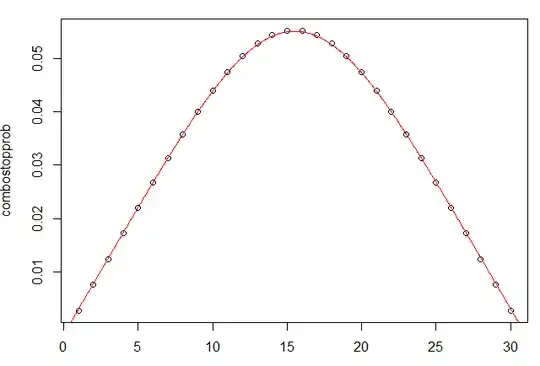
plot(combostopprob)
combostopprob
[1] 0.002772733 0.007675049 0.012473265 0.017251971 0.022004215 0.026704038
[7] 0.031310570 0.035766768 0.039998749 0.043916832 0.047418931 0.050396660
#[13] 0.052744012 0.054367815 0.055198392 0.055198392 0.054367815 0.052744012
#[19] 0.050396660 0.047418931 0.043916832 0.039998749 0.035766768 0.031310570
#[25] 0.026704038 0.022004215 0.017251971 0.012473265 0.007675049 0.002772733
sum(combostopprob) # should be 1
1

Jean Marie's simulation is very close to this.

This also gives the expected time.

sum(diff(c(0,probfinished[-t])) * 1:(t-1)) # expected time
# 403.0262
sum(1-c(0,probfinished)) # alternative
# 403.0262

The same code can equally well be used for larger $N$ - it just takes longer - or smaller $N$. Playing with that, there seems to be a limiting distribution after suitable rescaling as $N$ increases. I might guess it could be related to the distribution of the location of the first passage of a 2D Wiener process starting from the centre of a square boundary. Somebody asked that question on Reddit getting a general reply pointing at harmonic measure and another pointing at stochastic processes and boundary value problems.

Added: Damian Pavlyshyn's answer has since done that analysis. His limiting curve (with suitable rescaling) shown in red below fits these values in black very well, using

plot(combostopprob)
lines(t_grid*(N+1/3)+1/3, Re(dmu)/(N+1/3), col="red")