Optimal strategy for 1-player "snowball" game

Question

This particular game, which we can call "snowball", has one player and an operator who runs it.

It begins with an urn with one blue ball and one red ball inside.

The first round then starts, with each round working as follows:

• The operator picks a ball from the urn at random and both the operator and the player note its colour.
• The operator returns the ball to the urn and offers to add another ball of the same colour to the urn. The player can accept or reject the offer, ending the round.

At the end of $n$ rounds, a payout is given to the player based on the number of balls of the less frequent colour in the urn.

For example, here's one possibile outcome of game for $n = 5$, starting with 1 blue ball and 1 red ball in the urn:

• Operator picks out the blue ball and returns it, offering to add another blue ball. Player accepts. Urn now has 2 blue balls and 1 red ball.
• Operator picks out a blue ball and returns it, offering to add another blue ball. Player rejects. Urn now has 2 blue balls and 1 red ball.
• Operator picks out a red ball and returns it, offering to add another red ball. Player accepts. Urn now has 2 blue balls and 2 red balls.
• Operator picks out a red ball and returns it, offering to add another red ball. Player accepts. Urn now has 2 blue balls and 3 red balls.
• Operator picks out a red ball and returns it, offering to add another red ball. Player rejects. Urn now has 2 blue balls and 3 red balls.

The rounds now over, the player receives a payout of 2 as the minimum number of balls of a particular colour in the urn.

---

Is there an optimal strategy for a player of this game in terms of maximising the expected value of the payout after $n$ rounds? If so, what is it?

---

edit: There are two strategies one can immediately consider:

• Always accept, but if you do, it can quickly "snowball" out of control in favour of the majority colour since the probability increases of drawing more balls with that colour in future.

• Always reject when one colour would have two balls more than the other colour; this maintains the chances of drawing the minority colour in future, and returning to a balanced situation, but seems unnecessary for later rounds; e.g., adding a red ball to an urn with 100 blue balls and 101 red balls seems reasonable as the probability of drawing blue in future is not overly affected.

It seems that the second strategy of sometimes rejecting the majority colour to keep balance should be useful, but it's not clear what gap between both colours should be allowed. It seems the gap (in terms of number of balls) between the colours can be allowed to grow as the urn fills with more balls.

---

edit2: To add more context, I tried coding the two strategies with some quick-and-dirty code. I ran it for two colours and for the two strategies, now generalising the gap:

• Always accept.
• No gap of $z$: Reject when it would lead to one colour having $z$ more balls than the other. Otherwise accept.

The following is the average payout calculated over 1000 trials. The $x$-axis is the number of rounds run (up to 4096). The $y$-axis is the payout (count of minority colour).

So always accepting does not appear to be a good strategy. Having a look in more detail, in some cases the payout was single-digit for the always-accepting strategy after 4096 turns: there are cases where it "snowballs" towards a majority colour.

The optimal gap appears to depend on the number of rounds $n$, with larger gaps being better for larger $n$. Avoiding a gap of $4$ appears to be best for $n = 100$ (average payout $\sim 39.88$), while a gap of $24$ is best for $n = 4096$ (average payout $\sim 1958.29$).

---

edit3: Per a suggestion in a comment, I tried the following strategy:

• Keep minority percentage above $y$: Accept if both colours are tied. Otherwise reject when it would lead to one colour having below $y$% of the total balls; otherwise accept.

The optimal payouts are for $y = 48.0\%$ when $n = 4096$ (an average payout of $\sim 1966.59$) and $y = 39.8\%$ when $n = 100$ (an average payout of $\sim 40.52$). So the best percentage also appears to depend on $n$, growing as $n$ grows.

Answer 1

You can solve this as a Markov decision problem (stochastic dynamic programming) as follows. Let $D = \{\text{blue}, \text{red}\}$ be the set of two possible draws. Given $n$, let the states be $$\{(k,b,r,d): k \in \{0,\dots,n\}, b \in \{1,\dots,n+1\}, r \in \{1,\dots,n-k+2-b\}, d \in D\},$$ where $k$ is the number of remaining rounds, $b$ is the number of blue balls in the urn, $r$ is the number of red balls in the urn, and $d$ is the current draw. Let value function $V(k,b,r,d)$ denote the maximum expected payout. We want to compute $V(n,1,1,\text{blue})$, which is the same as $V(n,1,1,\text{red})$. The Bellman recursion is $$ V(k,b,r,d) = \begin{cases} \min(b,r) & \text{if $k = 0$} \\ \max\left(\frac{b+1}{b+1+r} V(k-1,b+1,r,\text{blue}) + \frac{r}{b+1+r} V(k-1,b+1,r,\text{red}), \\\frac{b}{b+r} V(k-1,b,r,\text{blue}) + \frac{r}{b+r} V(k-1,b,r,\text{red})\right) & \text{if $d = \text{blue}$} \\ \max\left(\frac{b}{b+r+1} V(k-1,b,r+1,\text{blue}) + \frac{r+1}{b+r+1} V(k-1,b,r+1,\text{red}), \\\frac{b}{b+r} V(k-1,b,r,\text{blue}) + \frac{r}{b+r} V(k-1,b,r,\text{red})\right) & \text{if $d = \text{red}$} \end{cases} $$

Here are the results for $n$ up to $100$:

The optimal expected payout for $n=100$ is approximately $41.47$.

Here's an animation of the optimal strategy when the draw is blue (the red draw strategy is just the opposite), where green means to accept and yellow means to reject: Looks like a linear separator would make a very good approximation.

---

By request, here's the animation when the draw is blue, but limited to only the states reachable from $(100,1,1,d)$ under the optimal strategy:

Answer 2

Summary

After some numerical investigation and heuristic arguments, I come to the following conclusions:

• The optimal value achievable is $n/2 - \Theta(\sqrt{n})$.
  • Numerically, it seems pretty close to $n/2 - \sqrt{n}$.
  • Theoretically, I have most of an argument that one can't do better than $n/2 - \Omega(\sqrt{n})$.
  • Theoretically, I have sketched an argument that one can achieve value $n/2 - O(\sqrt{n})$.
• A near-optimal policy is the square-root gap policy: when there are $k$ balls in the urn, accept a ball of the leading color if and only if the current gap is less than $\sqrt{k}$.
  • Numerically, I tried gap limits of the form $c \sqrt{k}$ for several constants $c$, and $c = 1$ appears to be the best for large $n$, with a suboptimality gap that remains much less than $1$.

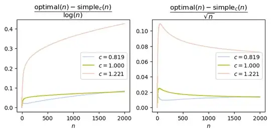
I conjecture that the square-root gap policy achieves expected value that is $o(\sqrt{n})$ less than the optimal value. I wouldn't be surprised if it were constant, because as of $n = 2000$, the suboptimality gap is still only $0.611$.

All code is included in an appendix.

Numerical investigations

Value of the optimal policy

Using dynamic programming, we can compute the optimal value of the optimal policy (along the lines of RobPratt's answer). The following two plots shows that $\text{optimal}(n)$, the value of the optimal policy, is (a) pretty close to $n/2$, and (b) the gap between them is slightly less than $\sqrt{n}$.

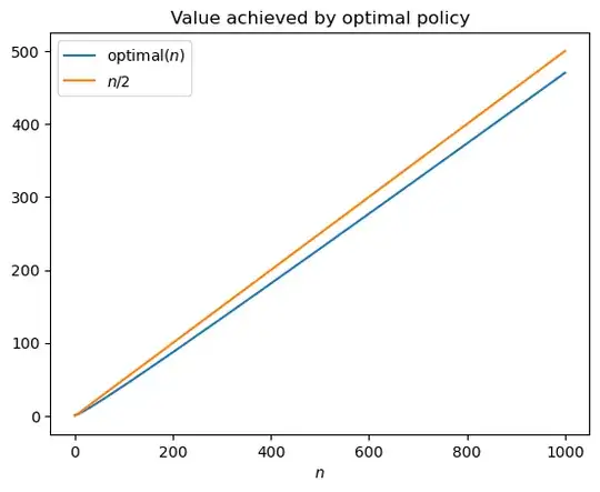
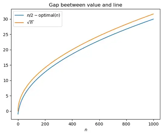
This is somewhat surprising: $n/2$ is the best we could possibly hope for, and we can achieve something pretty close to that. The fact that the value gap is $\sqrt{n}$ suggests that at the end, the gap between the colors is probably something like $\Theta(\sqrt{n})$ on average. This inspires a simple heuristic policy: always keep at most a square-root sized gap.

Simple heuristic: $c$-square-root gap policy

Let $\text{simple}_c(n)$ be the value of the $c$-square-root gap policy that operates as follows. Suppose there are $r$ red, $b$ blue, and $k = r + b$ total balls, and WLOG say $r > b$. The policy always accepts blue, but it only accepts red if $r - b < c \sqrt{k}$.

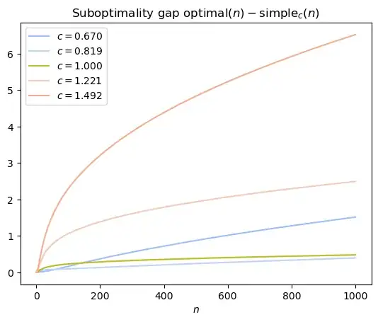
The following plots show that for a range of values of $c$, the $c$-square-root gap policy is pretty close to optimal. The specific case of $c = 1$ is highlighted yellow-green.

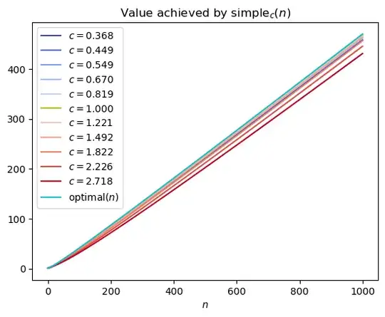
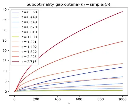
Zooming in on the best performers, it initially looks like $c < 1$ might outperform $c = 1$, but looking at larger values of $n$, it seems like $c = 1$ is the right choice asymptotically.

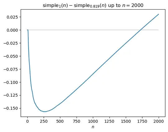
[update] Suboptimality gap of the $1$-square-root gap policy

I initially thought the suboptimality gap of the $1$-square-root policy might be constant. However, after making the plot below, I'm no longer fully convinced: it's conceivable that the gap is growing logarithmically, or even slightly faster. I do suspect it's still $o(\sqrt{n})$.

Heuristic arguments

There are two things we can argue theoretically:

• The optimal value is at most $n/2 - \Omega(\sqrt{n})$.
• One can achieve a value at least $n/2 - O(\sqrt{n})$.

I'm not going to write full proofs, though I believe turning these arguments into full proofs is possible.

Upper bound

Here's why the optimal value is at most $n/2 - \Omega(\sqrt{n})$. Imagine that every time step, we proposed adding red or blue each with probability $1/2$, instead of probabilities according to the current state. This increases the chance of proposing the trailing color, which should only help the optimal value. (This conclusion is the main thing that needs to be formalized.)

But now that we have equal-probability proposal colors, it never hurts to accept a ball, so we always accept. So the process becomes one driven by an unbiased random walk. Specifically, letting $S_n = \sum_{i = 1}^n B_i$ for $B_i \sim \operatorname{Uniform}\{-1, 1\}$ i.i.d., we have, by a central limit theorem approximation, $$ \text{optimal}(n) \leq \frac{n}{2} - \mathbb{E}[|S_n|] \approx \frac{n}{2} - \sqrt{\frac{2}{\pi} n}. $$

Lower bound

Here's a policy that I think achieves value at least $n/2 - O(\sqrt{n})$. It's a variant of the $c$-square-root gap policy, but with a change to make the dynamics mimic an unbiased random walk. Specifically, at every step:

1. If the $c$-square-root gap policy would reject a leading-color ball in this state, do the same.
2. If $c$-square-root gap policy would accept a leading-color ball in this state, then if a leading-color ball is drawn, reject it with some probability. Choose the probability such that the overall probability of accepting a leading-color ball equals that of accepting a trailing-color ball.

This means the number of balls evolves as a random walk with pauses, plus extra rejections from the gap hitting the $c \sqrt{k}$ barrier, where $k$ is the number of balls in the current state.

We now sketch why the number of rejections is at most $O(\sqrt{n})$. Because we keep a $c \sqrt{k}$ gap, this means the eventual value achieved is at least $n/2 - c \sqrt{k} - O(\sqrt{n}) = n/2 - O(\sqrt{n})$.

We first count the random rejections, those from list item 1 above. Because we're always maintaining a gap of at most $c \sqrt{k}$, the expected number of random rejections is $$ \mathbb{E}[\text{number of random rejections}] \leq \sum_{k = 2}^{n + 1} O\biggl(\frac{1}{\sqrt{k}}\biggr) \leq O(\sqrt{n}). $$ We should be able to use a concentration inequality to refine this into a high-probability statement. This means we're effectively running the $c$-square-root gap policy, but with equal-probability ball color proposals, for $n - O(\sqrt{n})$ steps.

To conclude, we need to argue that we only reject due to hitting the barrier $O(\sqrt{n})$ times, assuming equal-probability ball color proposals. I believe this is true but difficult to show. The rough idea is that an unbiased random walk will take, in expectation, $\ell - 1$ time to go from $1$ to either $0$ or $\ell$. This should mean that if we hit the barrier with $k$ balls in the urn, we'll reject some constant number of times to get away from the barrier, then take $\Omega(\sqrt{k})$ time in expectation until we next hit a barrier. Of course, the number of balls is increasing, but that should only further delay the time until the next barrier hit.

The above analysis can likely be adapted to the $c$-square-root gap policy without the random rejections, because the $\ell - 1$ hitting time should still approximately hold with slight bias in the walk. A policy that just uses random rejections with no barrier might also work, but one would need to show it doesn't get stuck in a state early on where it rejects a large number of leading-color balls.

Appendix: code

import numpy as np
import matplotlib.pyplot as plt
def dp_step_opt(v):
    """One step of dynamic programming, optimal policy
Parameters
----------
v : array of shape `(n, n)`
    Value function as a function of the number of reds and blues
    for some fixed number of time steps from the end.

Returns
-------
out : array of shape `(n - 1, n - 1)`
    Value function for one more time step from the end.
"""
v = np.asarray(v)
i = np.arange(v.shape[0] - 1)[:, np.newaxis]
j = np.arange(v.shape[1] - 1)[np.newaxis, :]
p = (i + 1) / (i + j + 2)
return (
    # v[i, j] == v[:-1, :-1]
    # v[i + 1, j] == v[1:, :-1]
    # v[i, j + 1] == v[:-1, 1:]
    p * np.maximum(v[:-1, :-1], v[1:, :-1])
    + (1 - p) * np.maximum(v[:-1, :-1], v[:-1, 1:])
)


def dp_step_simple(c, v=None):
    """One step of dynamic programming, simple square-root heuristic policy
Alternative usage: instead of `dp_step_simple(c, v)`,
can call as `dp_step_simple(c)(v)`.

Parameters
----------
c : float
    Constant for use in gap bound: when there are `k` balls in the urn,
    reject if the current gap is greater than `c * sqrt(k)`.

v : array of shape `(n, n)`
    Value function as a function of the number of reds and blues
    for some fixed number of time steps from the end.

Returns
-------
out : array of shape `(n - 1, n - 1)`
    Value function for one more time step from the end.
"""
if v is None:
    return lambda v: dp_step_simple(c, v)
v = np.asarray(v)
i = np.arange(v.shape[0] - 1)[:, np.newaxis]
j = np.arange(v.shape[1] - 1)[np.newaxis, :]
p = (i + 1) / (i + j + 2)
d_max = c * np.sqrt(i + j + 2)
return (
    # v[i, j] == v[:-1, :-1]
    # v[i + 1, j] == v[1:, :-1]
    # v[i, j + 1] == v[:-1, 1:]
    p * np.where(i - j >= d_max, v[:-1, :-1], v[1:, :-1])
    + (1 - p) * np.where(j - i >= d_max, v[:-1, :-1], v[:-1, 1:])
)


def dp(n, dp_step=dp_step_opt):
    """Dynamic programming for entire process
Parameters
----------
n : int
    Number of steps.

dp_step : callable, default=dp_step_opt
    One-step dynamic programming function, which encodes the policy used.

Returns
-------
out : list of arrays, `i`th of shape `(n + 1 - i, n + 1 - i)`
    Value functions for each number of time steps left.
    Overall value of the `i`-step game is `out[i][0, 0]`.
"""
i = np.arange(n + 1)[:, np.newaxis]
j = np.arange(n + 1)[np.newaxis, :]
vs = [1.0 + np.minimum(i, j)]
for _ in range(n):
    vs.append(dp_step(vs[-1]))
return vs


Value of optimal policy
dp_1000 = dp(1000)
v_opt = np.array([v[0, 0] for v in dp_1000])
ns = np.arange(len(v_opt))
Figure 1
plt.plot(v_opt, label=r"$\text{optimal}(n)$")
plt.plot(ns / 2, label="$n/2$")
plt.title("Value achieved by optimal policy")
plt.xlabel("$n$")
plt.legend()
plt.show()
Figure 2
plt.plot(ns / 2 - v_opt, label=r"$n/2 - \text{optimal}(n)$")
plt.plot(np.sqrt(ns), label=r"$\sqrt{n}$")
plt.title("Gap beetween value and line")
plt.xlabel("$n$")
plt.legend()
plt.show()
Value of simple policy
cvs_simple = [
    (c, np.array([v[0, 0] for v in dp(1000, dp_step=dp_step_simple(c))]))
    for c in np.exp(np.linspace(-1, 1, 11))
]
def color(c):
    if c == 1:
        return 'C8'
    else:
        return plt.get_cmap('coolwarm')(0.5 + 0.5 * np.log(c))
Figure 3
for c, v_simple in cvs_simple:
    plt.plot(v_simple, label=fr"$c = {c:.3f}$", color=color(c))
plt.plot(v_opt, label=r"$\text{optimal}(n)$", color='C9')
plt.title(r"$\text{Value achieved by }\text{simple}_c(n)$")
plt.xlabel("$n$")
plt.legend()
plt.show()
Figure 4
for c, v_simple in cvs_simple:
    plt.plot(v_opt - v_simple, label=fr"$c = {c:.3f}$", color=color(c))
plt.title(
    r"$\text{Suboptimality gap }\text{optimal}(n) - \text{simple}_c(n)$"
)
plt.xlabel("$n$")
plt.legend()
plt.show()
Value of simple policy, longer horizon
cvs_simple_2000 = [
    (c, np.array([v[0, 0] for v in dp(2000, dp_step=dp_step_simple(c))]))
    for c in np.exp(np.linspace(-1, 1, 11))[4:7]
]
Figure 6
plt.hlines(0, 2000, 0, color='lightgray')
plt.plot(cvs_simple_2000[1][1] - cvs_simple_2000[0][1])
plt.title(
    r"$\text{simple}1(n) - \text{simple}{0.819}(n)$ up to $n = 2000$"
)
plt.xlabel("$n$")
plt.show()
Estimating the suboptimality gap
dp_2000 = dp(2000)
v_opt_2000 = np.array([v[0, 0] for v in dp_2000])
ns_2000 = np.arange(len(v_opt_2000))
print(v_opt_2000[-1] - cvs_simple_2000[1][1][-1])
-> np.float64(0.6111886241664024)
Figure 7
plt.figure(figsize=(8, 3))
plt.subplot(1, 2, 1)
for c, v_simple in cvs_simple_2000:
    plt.plot(
        (v_opt_2000 - v_simple)[2:] / np.log(ns_2000[2:]),
        label=fr"$c = {c:.3f}$", color=color(c),
    )
plt.title(r"$\dfrac{\text{optimal}(n) - \text{simple}_c(n)}{\log(n)}$")
plt.xlabel("$n$")
plt.legend()
plt.subplot(1, 2, 2)
for c, v_simple in cvs_simple_2000:
    plt.plot(
        (v_opt_2000 - v_simple)[2:] / ns_2000[2:]**(1/2),
        label=fr"$c = {c:.3f}$", color=color(c),
    )
plt.title(r"$\dfrac{\text{optimal}(n) - \text{simple}_c(n)}{\sqrt{n}}$")
plt.xlabel("$n$")
plt.legend()
plt.show()