First observation: because the correlation structure of the $p$-values $Cor(P_n, P_m)$ depends on $n/m$, the time series often looks similar to the $p$-value time series above, no matter what the length of the time series is. It often has a lot of oscillation on the left hand side, and then it slows to moving slowly on the right hand side. E.g. this time series is 10 times longer than the one in the question but appears similar.

Secondly, there are simple approximate formulas for calculating $Cor(T_n, T_m)$ and $Cor(T_n^2, T_m^2)$, as Zach suggested.
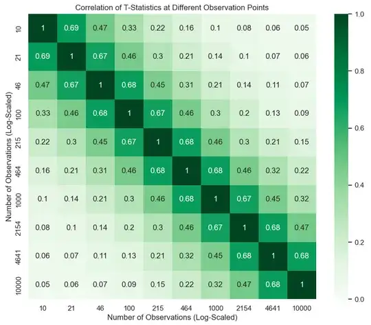
Claim: $Cor(T_n, T_m) \approx \sqrt{\frac{n}{m}}$.
Proof: The $t$-statistic is given by
$$T_n = \frac{\bar{X}_{1:n} - \bar{Y}_{1:n}}{s_{p}\sqrt{\frac{2}{n}}}$$
where
$$s_p = \sqrt{\frac{s_X^2 + s_Y^2}{2}}$$
Since $s_p \rightarrow 1$ in probability as $n \rightarrow \infty$, it is not an interesting term in the fraction because $\bar{X}_{1:n} - \bar{Y}_{1:n}$ and $\sqrt{\frac{2}{n}}$ both go to $0$. So we start by approximating the sample variance to just be $1$. So we are approximating $T_n \sim t_{2n-2}$ with $N(0, 1)$, which will be a good approximation or even fairly small $n$.
Assuming that $m > n$, the $t$-statistics can be written as
$$T_n = \frac{\bar{X}_{1:n} - \bar{Y}_{1:n}}{\sqrt{\frac{2}{n}}},\textrm{ and } T_m = \frac{\frac{n}{m}(\bar{X}_{1:n} - \bar{Y}_{1:n}) + \frac{1}{m}\sum_{i=n+1}^m(X_i - Y_i)}{\sqrt{\frac{2}{m}}}.$$
We need to compute
$$Cov(T_n, T_m) = \mathbb{E}(T_n T_m) - \mathbb{E}(T_n) \mathbb{E}(T_m).$$
$\mathbb{E}(T_n) = \mathbb{E}(T_m) = 0$, so we just need $\mathbb{E}(T_n T_m)$.
$$\mathbb{E}(T_n T_m) = \mathbb{E}\left(\frac{\bar{X}_{1:n} - \bar{Y}_{1:n}}{\sqrt{\frac{2}{n}}} \cdot \frac{\frac{n}{m}(\bar{X}_{1:n} - \bar{Y}_{1:n}) + \frac{1}{m}\sum_{i=n+1}^m(X_i - Y_i)}{\sqrt{\frac{2}{m}}}\right)$$
The observations up to $n$ and from $n + 1$ to $m$ are independent, so it simplifies to
$$\mathbb{E}(T_n T_m) = \frac{n\sqrt{nm}}{2m} \mathbb{E}\left[\left(\bar{X}_{1:n} - \bar{Y}_{1:n}\right)^2\right].$$
Here $\mathbb{E}\left[\left(\bar{X}_{1:n} - \bar{Y}_{1:n}\right)^2\right] = \frac{2}{n}$. Noting that $Var(T_n) = Var(T_m) = 1$, and performing cancellations, we have
$$Cov(T_n, T_m) = Cor(T_n, T_m) = \sqrt{\frac{n}{m}}.$$
If we look at the correlation of the $t$-statistics, we can see that this is a close fit empirically.
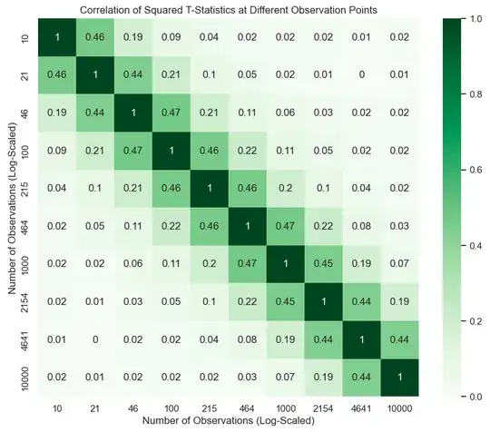
Claim: $Cor(T_n^2, T_m^2) \approx \frac{n}{m}$.
Proof:
$$Cor(T_n^2, T_m^2) = \frac{Cov(T_n^2, T_m^2)}{\sqrt{Var(T_n^2)Var(T_m^2)}}.$$
We already know the variances since we're approximating $T_n, T_m \sim N(0, 1)$, so $T_n^2, T_m^2 \sim \chi^2_1$, so $Var(T_n^2) = Var(T_m^2) = 2$.
$T_n, T_m$ are jointly normally distributed, and we can use the moments formula to get
$$\mathbb{E}\left(T_n^2 T_m^2\right) = Var(T_n)Var(T_m) + 2Cov(T_n, T_m)^2 = 1 + 2\frac{n}{m}.$$
Therefore
$$Cov(T_n^2, T_m^2) = \mathbb{E}\left(T_n^2T_m^2\right) - \mathbb{E}\left(T_n^2\right)\mathbb{E}\left(T_m^2\right) = \left[1 + 2\frac{n}{m}\right] - 1 = 2\frac{n}{m}.$$
Hence
$$Cor(T_n^2, T_m^2) = \frac{Cov(T_n^2, T_m^2)}{\sqrt{Var(T_n^2)Var(T_m^2)}} = \frac{n}{m}.$$
Again, this one is backed up by running simulations.
Thirdly, since the autocorrelation of the $t$-statistic and its square can be approximated by formulas of the form $\left(\frac{n}{m}\right)^k$, let's see if we can fit a formula of this form to the autocorrelation of the $p$-values. I computed a lot more $p$-value correlations (for each power of $10$ I calculated 25 correlations instead of the 3 I used in the correlation plots). I only kept ones that are above $0.1$, because I didn't run it with enough iterations to be confident of the values below this, and I'm about to do a log-transformation, when percentage error will make a big difference. I'm fitting the model $$Cor(P_n, P_m) = \left(\frac{n}{m}\right)^k,$$ so I take a log-transformation to both sides, getting
$$\log(Cor(P_n, P_m)) = k \log\left(\frac{n}{m}\right).$$
If I fit this regression with no intercept (to enforce $Cor(P_n, P_n) = 1$), I get the following fit.
 The slope is roughly $1.3$. It's not a perfect fit but I think it's a pretty good approximation, so I'll leave it at the empirically-estimated
$$Cor(P_n, P_m) \approx \left(\frac{n}{m}\right)^{1.3}.$$
The slope is roughly $1.3$. It's not a perfect fit but I think it's a pretty good approximation, so I'll leave it at the empirically-estimated
$$Cor(P_n, P_m) \approx \left(\frac{n}{m}\right)^{1.3}.$$


